
Action Recognition with Joints-Pooled 3D Deep Convolutional Descriptors
Proceedings of the Twenty-Fifth International Joint Conference on Artificial Intelligence. Pages 3324-3329.
Abstract
Torso joints can be considered as the landmarks of human body. An action consists of a series of body poses which are determined by the positions of the joints. With the rapid development of RGB-D camera technique and pose estimation research, the acquisition of the body joints has become much easier than before. Thus, we propose to incorporate joint positions with currently popular deep-learned features for action recognition. In this paper, we present a simple, yet effective method to aggregate convolutional activations of a 3D deep convolutional neural network (3D CNN) into discriminative descriptors based on joint positions. Two pooling schemes for mapping body joints into convolutional feature maps are discussed. The joints-pooled 3D deep convolutional descriptors (JDDs) are more effective and robust than the original 3D CNN features and other competing features. We evaluate the proposed descriptors on recognizing both short actions and complex activities. Experimental results on real-world datasets show that our method generates promising results, outperforming state-of-the-art results significantly.
- [Cao et al., 2015] Congqi Cao, Yifan Zhang, and Hanqing Lu. Spatio-temporal triangular-chain CRF for activity recognition. In ACM MM, pages 1151-1154, 2015.
- [Chen et al., 2011] Cheng Chen, Yueting Zhuang, Feiping Nie, Yi Yang, Fei Wu, and Jun Xiao. Learning a 3d human pose distance metric from geometric pose descriptor. IEEE Trans. Vis. Comput. Graph., 17(11):1676-1689, 2011.
- [Chéron et al., 2015] Guilhem Chéron, Ivan Laptev, and Cordelia Schmid. P-CNN: pose-based CNN features for action recognition. CoRR, abs/1506.03607, 2015.
- [Dalal and Triggs, 2005] Navneet Dalal and Bill Triggs. His- tograms of oriented gradients for human detection. In CVPR, pages 886-893, 2005.
- [Dalal et al., 2006] Navneet Dalal, Bill Triggs, and Cordelia Schmid. Human detection using oriented histograms of flow and appearance. In ECCV, pages 428-441, 2006.
- [Du et al., 2015] Yong Du, Wei Wang, and Liang Wang. Hi- erarchical recurrent neural network for skeleton based ac- tion recognition. In CVPR, pages 1110-1118, 2015.
- [Fan et al., 2008] Rong-En Fan, Kai-Wei Chang, Cho-Jui Hsieh, Xiang-Rui Wang, and Chih-Jen Lin. LIBLINEAR: A library for large linear classification. Journal of Machine Learning Research, 9:1871-1874, 2008.
- [Hariharan et al., 2015] Bharath Hariharan, Pablo Andrés Arbeláez, Ross B. Girshick, and Jitendra Malik. Hyper- columns for object segmentation and fine-grained local- ization. In CVPR, pages 447-456, 2015.
- [Jhuang et al., 2013] Hueihan Jhuang, Juergen Gall, Silvia Zuffi, Cordelia Schmid, and Michael J. Black. Towards un- derstanding action recognition. In ICCV, December 2013.
- [Ji et al., 2013] Shuiwang Ji, Wei Xu, Ming Yang, and Kai Yu. 3d convolutional neural networks for human action recognition. IEEE Trans. Pattern Anal. Mach. Intell., 35(1):221-231, 2013.
- [Karpathy et al., 2014] Andrej Karpathy, George Toderici, Sanketh Shetty, Thomas Leung, Rahul Sukthankar, and Fei-Fei Li. Large-scale video classification with convolu- tional neural networks. In CVPR, pages 1725-1732, 2014.
- [Laptev et al., 2008] Ivan Laptev, Marcin Marszalek, Cordelia Schmid, and Benjamin Rozenfeld. Learning realistic human actions from movies. In CVPR, 2008.
- [Lillo et al., 2014] Ivan Lillo, Alvaro Soto, and Juan Carlos Niebles. Discriminative hierarchical modeling of spatio- temporally composable human activities. In CVPR, pages 812-819, 2014.
- [Nie et al., 2015] Bruce Xiaohan Nie, Caiming Xiong, and Song-Chun Zhu. Joint action recognition and pose estima- tion from video. In CVPR, pages 1293-1301, 2015.
- [Shotton et al., 2013] Jamie Shotton, Toby Sharp, Alex Kip- man, Andrew W. Fitzgibbon, Mark Finocchio, Andrew Blake, Mat Cook, and Richard Moore. Real-time human pose recognition in parts from single depth images. Com- mun. ACM, 56(1):116-124, 2013.
- [Simonyan and Zisserman, 2014] Karen Simonyan and An- drew Zisserman. Two-stream convolutional networks for action recognition in videos. CoRR, abs/1406.2199, 2014.
- [Tompson et al., 2014] Jonathan Tompson, Arjun Jain, Yann LeCun, and Christoph Bregler. Joint training of a convo- lutional network and a graphical model for human pose estimation. CoRR, abs/1406.2984, 2014.
- [Tran et al., 2014] Du Tran, Lubomir D. Bourdev, Rob Fer- gus, Lorenzo Torresani, and Manohar Paluri. C3D: generic features for video analysis. CoRR, abs/1412.0767, 2014.
- [Wang and Schmid, 2013] Heng Wang and Cordelia Schmid. Action Recognition with Improved Trajectories. In ICCV, pages 3551-3558. IEEE, December 2013.
- [Wang et al., 2011] Heng Wang, A. Klaser, C. Schmid, and Cheng-Lin Liu. Action recognition by dense trajectories. In CVPR, pages 3169-3176, 2011.
- [Wang et al., 2013] Heng Wang, Alexander Kläser, Cordelia Schmid, and Cheng-Lin Liu. Dense trajectories and mo- tion boundary descriptors for action recognition. Interna- tional Journal of Computer Vision, 103(1):60-79, 2013.
- [Wang et al., 2014] Jiang Wang, Xiaohan Nie, Yin Xia, Ying Wu, and Song-Chun Zhu. Cross-view action modeling, learning, and recognition. In CVPR, pages 2649-2656, 2014.
- [Wang et al., 2015] Limin Wang, Yu Qiao, and Xiaoou Tang. Action recognition with trajectory-pooled deep- convolutional descriptors. In CVPR, pages 4305-4314, 2015.
- [Yang and Ramanan, 2011] Yi Yang and Deva Ramanan. Ar- ticulated pose estimation with flexible mixtures-of-parts. In CVPR, pages 1385-1392, 2011.
- [Zhang et al., 2013] Weiyu Zhang, Menglong Zhu, and Kon- stantinos G. Derpanis. From actemes to action: A strongly-supervised representation for detailed action un- derstanding. In ICCV, pages 2248-2255, 2013.
References were extracted automatically from the PDF and may contain errors.
Full text extracted automatically from the PDF; figures, tables and equations may differ. The PDF is the version of record.
1 Introduction
Recognizing the action performed in video is one of the most popular research field in computer vision. Different from images which only contain spatial information, videos are three dimensional (3D) spatio-temporal flow. A lot of research focused on how to take both the appearance and motion information into account for video-based action recognition.
Much of the initial work on action recognition used handcrafted features such as HOG [Dalal and Triggs, 2005], HOF [Dalal et al., 2006], STIP [Laptev et al., 2008], Dense Trajectories (DT) [Wang et al., 2011] and Improved Trajectories (iDT) [Wang and Schmid, 2013]. Dense trajectories are shown to be an effective video representation for action recognition. By taking camera motion into consideration, iDT improves the performance further.
⇤Corresponding author
Besides trajectories of dense points, human action can be represented by the trajectories of body joints which is more discriminative and compact. Currently, reliable joint coordinates can be obtained by using the real-time skeleton estimation algorithms [Tompson et al., 2014] [Shotton et al., 2013]. Most of the existing skeleton-based action recognition methods model the temporal dynamics of body joints with handcrafted features, such as the relative location between body joints, angles between limbs and angles between limbs and planes spanned by body parts [Chen et al., 2011]. However, these methods can not deal with the situations with similar spatial and temporal variations of body joints, such as "grab" and "deposit" [Du et al., 2015], because the surrounding information around the joints is lost. Another limitation of existing skeleton-based method is that they can not handle the self-occlusion and error body joints explicitly.
Encouraged by the success of CNNs in image classification, recently much effort is spent on applying CNNs to video-based action recognition. There are mainly two ways of applying CNNs on video data. One is using the 2D CNN architecture. Directly applying image-based models to individual frames of videos can only characterize the visual appearance. The two-stream CNN architecture [Simonyan and Zisserman, 2014] learns motion information by using an additional 2D CNN which takes the optical flow as input. The stacked optical flow frames are treated as different channels.
After convolutional operation, the temporal dimension is collapsed completely. Therefore the two-stream CNN is less effective for characterizing long-range motion patterns in multiple frames.
The other way of adapting CNNs to video is using 3D CNNs with 3D convolution and 3D pooling layers [Karpathy et al., 2014; Ji et al., 2013; Tran et al., 2014]. 3D convolution layer takes a volume as input and outputs a volume which preserves the temporal information of the input. Both spatial information and temporal information are abstracted layer by layer. The features used in [Tran et al., 2014] are from fully-connected layers of a 3D CNN named C3D. Compared to fully-connected layers, 3D convolution layers retain 3D spatio-temporal structure. Different convolution layers provide bottom-up hierarchical semantic abstraction. In image-based computer vision tasks, there have been explorations to utilize multiple convolution layers for classification [Hariharan et al., 2015]. It is worth exploring how to utilize spatio-temporal information in 3D convolution layers to obtain features which combine different levels of abstraction.
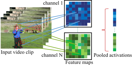
Inspired by the trajectory-pooled deep convolutional descriptors (TDDs) [Wang et al., 2015] which used dense trajectory points to pool 2D CNN feature maps. We propose an efficient way of pooling activations in 3D feature maps based on joint positions to generate video descriptors as illustrated in Figure 1. The features are called joints-pooled 3D deep convolutional descriptors (JDDs). When mapping points from video into feature maps, TDD and JDD use two different mapping methods. TDD used ratio scaling to map points, in which only the sizes of input and output are considered. We compute the corresponding points with the concept of receptive field, which is more appropriate.
The idea of JDD is different from another pose-based CNN descriptor P-CNN [Ch´eron et al., 2015] which crops RGB and optical flow images into multiple part patches (e.g. right hand and left hand) as the inputs of a two-stream CNN. Instead of using multiple inputs, we take advantage of the abundant information in 3D convolutional feature maps by joints pooling. Our approach is more efficient in computation than P-CNN which needs to compute not only body joints but also optical flow and uses multiple inputs with two deep 2D CNNs. Furthermore, we do not need to compute activations of fully-connected layers.
The main procedures of our framework are as follows:
1) Split videos to fixed-length clips. 2) Compute 3D convolutional feature maps for each clip. 3) Use the annotated or estimated joints of the video to localize points in the 3D feature maps of a convolution layer. 4) Pool out the activations at each corresponding point. 5) Concatenate all the pooled activations in the same clip together. 6) Use average pooling and L2 normalizaiton to aggregate clip features into video features. 7) Use linear SVM to do classification.
The main contributions of our work include:
- ÷ We are the first to combine 3D CNNs and body joints to improve action recognition by using joint positions to pool convolutional activations. Even with estimated joint positions which are not as accurate as manually annotated data, the experimental results are still promising, outperforming other features.
- ÷ We use a novel method to map the joint positions in videos to points in feature maps for pooling by taking kernel sizes, stride values and padding sizes of 3D CNN layers into account which is more appropriate than directly using ratio scaling.
- ÷ The simple, yet effective convolutional feature map pooling method has better generalization ability than the original C3D feature. It can apply to novel datasets without carefully-designed finetuning and get better performance than C3D.
2 Joints-pooled 3DDeep Convolutional Descriptors
In this section, firstly, we review the 3D architecture proposed in [Tran et al., 2014]. Then we describe the concepts of receptive field and corresponding points in 3D convolutional networks. Finally we introduce two methods of mapping joint positions to the coordinates in convolutional feature maps.
2.1 3DConvolutional Networks Revisited
We use the C3D model trained on Sports-1M provided by [Tran et al., 2014] to compute 3D convolutional feature maps.
Using shorthand notation, the full architecture of C3D is conv1a(64)-pool1-conv2a(128)-pool2-conv3a(256)- conv3b(256) - pool3 - conv4a(512) - conv4b(512) - pool4- conv5a(512) - conv5b(512) -pool5- f c6(4096) - fc7(4096)-softmax, where the number in parenthesis indicates the number of convolutional filters. All 3D convolution kernels are 3 ⇥ 3 ⇥ 3 (in the manner of k ⇥ k ⇥ d, where k is spatial size and d is temporal depth) with stride 1 and padding 1 in both spatial and temporal dimensions. All pooling kernels are 2⇥2⇥2, except for pool1 which is 2⇥2⇥1 with the intention of not to merge the temporal signal too early. C3D takes a clip of 16 frames as input. It resizes the input frames to 171⇥128 (width ⇥ height), then crops to 112⇥112. More details and explanations can be found in [Tran et al., 2014].
Compared with C3D which used fc6 as features, the proposed approach does not need to compute activations of any fully-connected layer since it pools on convolutional layers.
2.2 3DReceptive Field and Coordinate Mapping
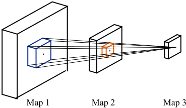
In CNNs, receptive field is an important concept, which embodies a particular region of sensory space between layers. The receptive field of 3D CNNs is a spatio-temporal cube instead of a spatial rectangle for 2D CNNs.
As illustrated in Figure 2, after the operation of convolution or pooling, a point in Map3 corresponds to a cube in Map2 which is enclosed with red lines. And the cube in Map2 corresponds to an bigger cube in Map1 which is enclosed with blue lines. Therefore, the point inMap3 actually corresponds to the cube enclosed with the blue lines in Map1. The size of receptive field can be computed layer by layer.
Besides receptive field, we can obtain the mapping relationship of points between layers. Let pi be a point in the ith layer. (xi↪ yi↪ ti) is the coordinate of pi. Given pi+1, the corresponding point pi can be computed by mapping pi+1 back to the ith layer. Actually, pi is the center point of the receptive field corresponding to pi+1.
For the convolution layers and pooling layers:
where sxi ↪ kx i ↪ paddingx i are the x-axis component of stride, kernel size and padding of the ith layer respectively. The equation also applies to y and t dimensions. Note that for 3D CNNs, the operations of convolution layers and pooling layers not only act on spatial dimensions, but also act on temporal dimension. Therefore the kernel size, stride and padding value are three dimensional.
For ReLU layers:
Reversely, given the coordinate of pi, we can compute the coordinate of pi+1. The point pi+1 corresponds to a receptive field in the ith layer, while the receptive field takes pi as the center.
2.3 Joints PoolingMethods
For JDD, we compare two ways of pooling 3D convolutional activations based on different schemes for mapping body joints into convolutional feature maps. One is using the ratio of output to input in spatial and temporal dimensions to scale the joint coordinates into feature maps as below, which is named as Ratio Scaling.
where (xic ↪ yic ↪ tic ) is the point coordinate in the ith 3D convolutional feature maps corresponding to (xv↪ yv↪ tv) which is the joint coordinate in video. (rix ↪ riy ↪ ri t ) is the ratio of the ith convolutional feature maps to the video in spatial and temporal dimensions.
The other way is using the equations of computing receptive field and mapping points with 3D convolutional and pooling operations described in Section 2.2. With this method we need to compute the corresponding points of joints by taking kernel sizes, strides and padddings of all the preceding layers into account. We call this method Coordinate Mapping.
After bringing the values of C3D kernel sizes 3 ⇥ 3 ⇥ 3, strides 1 (in spatial and temporal dimensions) and paddings 1 into Equation 1, we can see that the convolution layers in C3D do not change the coordinates of mapping points between layers.
A pooling layer with kernel size 2 ⇥ 2 ⇥ 2 and stride 1 changes the coordinate between input and output feature maps as follows.
We need to take all the preceding layers into consideration to compute the coordinate mapping relationship between feature maps and video. Specifically, the relationship between points coordinate in the ith convolutional feature maps and joint positions in video is as follows.
Note that there is a little difference in temporal dimension because the kernel size of pool1 is 2⇥2⇥1 with the intention of not to merge the temporal signal too early.
Since we can use body joints in video to localize points in 3D feature maps, we can pool out the activations at each corresponding point. All the pooled activations belonging to the same clip are concatenated together. Average pooling and L2 normalization are used to aggregate clip features into video features. The dimension of JDD is C ⇥ L ⇥ N, where C is the number of feature map channels, L is the length of the video clip which is 16 in our experiments, N is the number of body joints in each frame.
The JDDs from different convolutional layers can be fused together to improve performance due to complementarity. JDD can also be combined with other features or models.
3 Experiments
In this section, Firstly, we make a brief introduction to the datasets we use. Then, we describe the exploratory experiments we make to compare the two pooling schemes. We also test the robustness of JDD with inaccurate estimated joints. Finally, we evaluate JDDs on public datasets and give the comparison to the state-of-the-art results.
3.1 Datasets
We evaluate our method on three public action datasets: subJHMDB [Jhuang et al., 2013], Penn Action [Zhang et al., 2013] and Composable Activities [Lillo et al., 2014]. These datasets cover indoor and outdoor actions.
sub-JHMDB dataset is a subset of JHMDB with full body inside the frame, containing 316 videos with 12 action categories. sub-JHMDB provides action labels and 15 body joints for each frame. We use the 3-fold cross validation setting provided by the dataset for experiments. The dataset is collected from movies or Internet. The lengths of frames in videos ranges from 16 to 40.
Penn Action dataset contains 2326 video sequences of 15 different actions and annotations of 13 body joints for each sequence. There are videos in which not all the body joints are visible. We use the 50/50 trainning/testing split provided by the dataset to do experiments. The videos are obtained from various online video repositories. The lengths of frames in videos is from 18 to 663.
| Concatenate all the activations | JDD Ratio Scaling (1 ⇥ 1 ⇥ 1) | JDD Coordinate Mapping (1 ⇥ 1 ⇥ 1) | JDD Ratio Scaling (3 ⇥ 3 ⇥ 3) | JDD Coordinate Mapping (3 ⇥ 3 ⇥ 3) | |
|---|---|---|---|---|---|
| joint coordinates | 0.4565 | - | - | - | - |
| fc7 | 0.6771 | - | - | - | - |
| fc6 | 0.6884 | - | - | - | - |
| conv5b | 0.6702 | 0.7570 | 0.8186 | 0.7843 | 0.7919 |
| conv5a | 0.5952 | 0.7246 | 0.7343 | - | - |
| conv4b | 0.5057 | 0.7272 | 0.7251 | 0.7427 | 0.7767 |
| conv4a | 0.4667 | 0.7439 | 0.7063 | - | - |
| conv3b | 0.3943 | 0.6532 | 0.6385 | 0.6730 | 0.6733 |
Composable Activities dataset consists of 693 videos containing activities in 16 classes performed by 14 actors. Each activity is composed by spatio-temporal combinations of atomic actions. Note that there is no ground-truth joints in this dataset. We use the estimated body joints extracted from RGB-D videos provided by [Lillo et al., 2014]. The videos are relatively long compared to the other two datasets. The lengths of frames in videos is from 83 to 1351.
3.2 Implementation details
For Penn Action and Composable Activities datasets, the videos are split into 16-frame long clips with 8-frame overlap between two consecutive clips as inputs of C3D. For subJHMDB, due to its short length in time, we split each video to three clips which are the first 16 frames, the middle 16 frames and the last 16 frames.
Each clip is input to C3D. We pool the activations in a particular 3D convolution layer out based on joint positions. The activations pooled out are concatenated to be the descriptor of the input clip. For sub-JHMDB and Penn Action datasets, the descriptors of clips are averaged to form a video descriptor which is normalized by L2-norm. Linear SVM [Fan et al., 2008] is used to classify the videos. For long-time videos in Composable Activities dataset, we use HMMs to do classification which will be described in Section 3.7.
On sub-JHMDB and Penn Action datasets, we do not finetune C3D. For Composable Activities dataset, which is much different from Sports-1M, we finetune the network with a few iterations (see Section 3.7 for specific experimental settings).
3.3 Analysis of JDD and baselines
In this section, we compare JDD with joint coordinates and C3D features [Tran et al., 2014]. We also show the experiments on pooling different 3D convolution layers with different joints mapping algorithms. We experiment on subJHMDB without finetuning. Firstly, we test the C3D features. The recognition accuracy of fc6, fc7 and flattened convolutional activations are listed in the first column of Table 1. The results verify that deep architectures learn multiple levels of abstraction layer by layer.
We test JDD with pooling one activation on the corresponding point in feature maps and pooling a 3 ⇥ 3 ⇥ 3 cube around the corresponding point with Ratio Scaling and Coordinate Mapping introduced in Section 2.3. The recognition results are shown in Table 1. We can see that, compared with C3D features, our JDDs have superior performance which demonstrates the effectiveness of joints pooling. Generally, the higher layers encapsulate more discriminative information for recognition. Pooling a cube around the mapping points is usually better than pooling one activation because the former takes more surrounding information into account, except for conv5b. It is probably because that the spatial and temporal size of feature maps in conv5b is small, thus a cube around the mapping points encloses too much global information which impairs the performance. At shallow layers, JDD Ratio Scaling and JDD Coordinate Mapping are very close in performance. As the layer goes deeper, the performance of Coordinate Mapping is much better than Ratio Scaling. It is probably because that the difference between the coordinates of mapping points obtained by the two methods is bigger and bigger with the increase of layers, while the influence of kernel sizes, strides and paddings of layers is more and more significant. The best result is obtained by JDD of conv5b with Coordinate Mapping. For other layers, pooling a cube around the corresponding point computed with Coordinate Mapping is better than with Ratio Scaling. Coordinate Mapping is more appropriate than Scaling Ratio. We use 1 ⇥ 1 ⇥ 1 Coordinate Mapping for conv5b and 3 ⇥ 3 ⇥ 3 Coordinate Mapping for conv4b in the rest experiments.
If we use max-pooling to down sample the feature maps into responses of windows, then accumulate the responses into a descriptor, the accuracy is 0▷7047 for conv5, which is higher than fc6 and flattened conv5 features, while much lower than JDDs. This demonstrates that convolution layers contain spatio-temporal information and body joints are important for human action recognition. Our JDD does make full use of spatial and temporal information learned by C3D and utilize body joints to omit irrelevant information in the background.
| Method | GT | Esti | Diff |
|---|---|---|---|
| JDD (conv5b) | 0.819 | 0.777 | 0.042 |
| P-CNN [Ch´eron et al., 2015] | 0.725 | 0.668 | 0.057 |
| Pose [Jhuang et al., 2013] | 0.751 | 0.529 | 0.222 |
| HLPF [Yang and Ramanan, 2011] | 0.782 | 0.511 | 0.271 |
3.4 Evaluation on sub-JHMDB Datasets
In this section, we compare our method with other published methods. To evaluate the influence of joints precision to JDD, we generate JDD based on the estimated joints provided by [Yang and Ramanan, 2011]. The accuracies of JDD based on ground-truth joints and estimated joints are listed in Table 2. The drop of accuracy is also reported. We compare JDD with P-CNN [Ch´eron et al., 2015], Pose [Jhuang et al., 2013] and HLPF [Yang and Ramanan, 2011]. P-CNN is a pose-based CNN descriptor which uses positions of body joints to crop RGB and optical flow images into patches; The activations of CNN fully-connected layer produced by multiple patches are aggregated to describe the input video. Pose and HLPF are two kinds of hand-crafted high-level pose features.
From Table 2, we can see that JDD outperforms the-stateof-the-art results significantly on sub-JHMDB. Note that we only use the JDD pooled from conv5b layer and use simple averaging pooling between clips. JDD achieves the best performance not only on ground-truth joints, but also on estimated joints, exceeding other methods in the order of 10%. And the drop of accuracy for JDD is the smallest among all the descriptors which demonstrates that JDD is robust to errors in pose estimation. If we use max+min pooling in temporal dimension as [Ch´eron et al., 2015], the JDD accuracy of conv5b could be further improved to 82.6%.
The superior performance of JDD compared to P-CNN demonstrates that we do not need to crop the images into multiple patches to advance accuracy as usual. The information in feature maps produced by taking one image or video clip as input is abundant. We can take good advantage of it by joints pooling.
3.5 Analysis of Feature Fusion
As mentioned above, the receptive field of a particular point in convolutional feature maps is a cube which corresponds to a spatio-temporal region in video. With the increase of convolution layers, spatial and temporal information is abstracted from the parts to the whole. Different layers pick up discriminative information at different abstract level. We try to fuse JDDs from different layers together to see if they can compensate each other. We also test the fusion of JDD and other features. Table 3 represents the results of different combinations of features using late fusion by the scores of SVM. The combination of JDDs of conv5b and conv4b improves the performance mostly. Higher accuracy should be obtained by fusing more complementary information together.
| Fusion Layers | Accuracy |
|---|---|
| JDD (conv5b+fc6) | 0.825 |
| JDD (conv5b+conv4b) | 0.833 |
| JDD (conv5b+conv3b) | 0.830 |
| JDD (conv5b+joint coordinates) | 0.819 |
3.6 Evaluation on Penn Action Dataset
On Penn Action dataset in which there are videos with invisible body joints, compared to other methods, JDD also achieves the best accuracy as shown in Table 4.
We use the algorithm in [Yang and Ramanan, 2011] to generate estimated joints in Penn Action dataset without finetuning. The per joint L1 distance error (pixels) between the ground-truth joints and estimated joints is (68.52, 40.67) in width and height. Note that the authors of [Nie et al., 2015] removed the action "playing guitar" and several other videos because less than one third of a person is visible in those data. While we do not remove any videos. This illustrates that JDD is robust for occlusion. The authors [Nie et al., 2015] also corrected errors of un-annotated joints by training a regression model to predict their positions. While we do nothing to rectify the positions of joints. We even do not finetune the skeleton estimation algorithm on Penn Action dataset. This indicates that JDD is not sensitive to error joints.
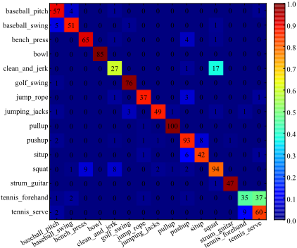
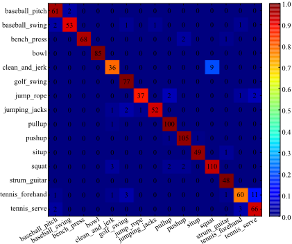
We visualize the confusion matrixes obtained by C3D fc6 feature and JDD from conv5b in Figure 3 and Figure 4 respectively. We can see that the most confusing categories are "clean and jerk" with "squat", "tennis forehand" with "tennis serve" due to their similarity in appearance and motion. By the ability to extract more discriminative spatio-temporal information, JDD performs better than C3D fc6 features.
If we use max+min pooling in time as [Ch´eron et al., 2015] instead of average pooling, the JDD accuracy of conv5b could be further improved to 97.1% and the accuracy of fusing conv5b and conv4b could be 98.1%.
The promising results indicate that JDD is not limited to the situations with full human joints visible. We also do experiments on the full JHMDB dataset in which two thirds of the videos contain joints annotated outside the frames. The best result of JDDs is 72.63%. We believe that if we add more proper operations to handle the case of outside joints instead of simply mapping those points to their nearest points on the image edge as we do now, the performance could be further improved.
3.7 Evaluation on Composable Activities Dataset
For Composable Activities dataset, there are 14 actors. Following the same experimental settings as [Lillo et al., 2014], performance is evaluated with leave-one-subject-out. Because the number of clips of this dataset is relatively large, and this dataset is indoor human activities composed of temporal and spatial arrangement of actions which is much different from the pre-trained Sports-1M dataset, we finetune C3D. For different splits, we use the same finetuning settings. We do finetuning using mini-batches of 30 clips, with learning rate of 0.0003. The finetuning is stopped after 5000 iterations. Linear SVM is used for action classification. As for activity recognition, we use HMMs with 6 hidden states to model the dynamic of the whole video sequence. C3D fc6 and JDD features are firstly reduced to 64 dimensions with PCA to reduce the model complexity.
The ground-truth action labels are annotated to each part of human body (e.g. left arm and right leg). Thus, the labels could be overlapped at a frame such as "waving hand" and "walking". For these situations, we simply use a label of one body part as the label of 16-frame clip to train SVM. The recognition accuracy of action is 56.3% and 55.2% for C3D fc6 and JDD from conv5b respectively. The competing methods used complex graph models with multiple chains to model different body parts. With 4 chains corresponding to 4 body parts, the action accuracies for Hierarchical Model [Lillo et al., 2014] and ST TriCRF [Cao et al., 2015] are 70.2% and 56.6% respectively. However, the action accuracy is much lower for ST TriCRF [Cao et al., 2015] which is 33.8% when dealing with overlapping frames as us. We can also aggregate activations pooled out by body joints belong to the same body part to generate part descriptors. By using complex graph models to model different body parts, the accuracy of JDD could be improved further.
| Method | Accuracy |
|---|---|
| STIP [Zhang et al., 2013] | 0.829 |
| Dense [Wang et al., 2013] | 0.734 |
| MST [Wang et al., 2014] | 0.740 |
| Action Bank [Zhang et al., 2013] | 0.839 |
| Actemes [Zhang et al., 2013] | 0.794 |
| Graph Model [Nie et al., 2015] | 0.855 |
| C3D (fc6) | 0.860 |
| JDD (estimated joints)(conv5b) | 0.874 |
| JDD(conv5b) | 0.943 |
| JDD(conv5b+conv4b) | 0.957 |
| Method | Accuracy |
|---|---|
| BoW [Lillo et al., 2014] | 0.672 |
| H-BoW [Lillo et al., 2014] | 0.742 |
| HMM [Lillo et al., 2014] | 0.765 |
| Hierarchical Model [Lillo et al., 2014] | 0.857 |
| ST TriCRF [Cao et al., 2015] | 0.790 |
| C3D (fc6) | 0.860 |
| JDD (estimated joints) (conv5b) | 0.879 |
The recognition accuracy of activity is shown in Table 5. Except C3D, the other competing methods used hand-crafted skeleton features. Note that with HMMs, the accuracy of the skeleton features in [Lillo et al., 2014] is 76.5% which is much lower than 87.9% of JDD. Even with complex graph models, the accuracy of skeleton features can not exceed JDD. As we can see, C3D is a powerful feature extractor for recognition. With the estimated pose information, our proposed JDD gets the highest accuracy even with a low dimension after PCA which demonstrates that JDD is an effective, robust and scalable descriptor for videos.
4 Conclusions
We propose a novel joints-pooled 3D deep convolutional descriptor (JDD) in this paper which can take advantages of body joints and C3D. Body joints are expressive features of human pose. C3D is a generic model to extract spatiotemporal information in videos. We utilize body joints to sample discriminative points from feature maps generated by C3D. Promising experimental results in indoor / outdoor, short-time / long-time datasets with annotated / estimated joints demonstrate the effectiveness and robustness of JDD in video-based human action recognition.
5 Acknowledgments
We thank the anonymous reviewers for their valuable comments. This work was partly supported by 863 Program (2014AA015104) and National Natural Science Foundation of China (61332016, 61572500, 61379100,61303154).
@inproceedings{ijcai2016p470,
  title     = {Action Recognition with Joints-Pooled 3D Deep Convolutional Descriptors},
  author    = {Cao, Congqi and Zhang, Yifan and Zhang, Chunjie and Lu, Hanqing},
  booktitle = {Proceedings of the Twenty-Fifth International Joint Conference on
               Artificial Intelligence, {IJCAI-16}},
  publisher = {AAAI Press / International Joint Conferences on Artificial Intelligence},
  editor    = {Subbarao Kambhampati},
  pages     = {3324--3329},
  year      = {2016},
  month     = {7},
  url       = {https://ijcai.org/proceedings/2016/470},
}
TY - CPAPER TI - Action Recognition with Joints-Pooled 3D Deep Convolutional Descriptors AU - Cao, Congqi AU - Zhang, Yifan AU - Zhang, Chunjie AU - Lu, Hanqing T2 - Proceedings of the Twenty-Fifth International Joint Conference on Artificial Intelligence, IJCAI-16 PB - AAAI Press / International Joint Conferences on Artificial Intelligence PY - 2016 SP - 3324 EP - 3329 UR - https://ijcai.org/proceedings/2016/470 ER -Copied
Machine-readable versions of this paper, for tools and AI agents:





