
Saliency Transfer: An Example-Based Method for Salient Object Detection
Proceedings of the Twenty-Fifth International Joint Conference on Artificial Intelligence. Pages 3411-3416.
Abstract
Over the past decades, numerous theories and studies have demonstrated that salient objects in different scenes often share some properties in common that make them visually stand out from their surroundings, and thus can be processed in finer details. In this paper, we propose a novel method for salient object detection that involves the transfer of the annotations from an existing example onto an input image. Our method, which is based on the low-level saliency features of each pixel, estimates dense pixel-wise correspondences between the input image and an example image, and then integrates high-level concepts to produce an initial saliency map. Finally, a coarse-to-fine optimization framework is proposed to generate uniformly highlighted salient objects. Qualitatively and quantitatively experiments on six popular benchmark datasets validate that our approach greatly outperforms the state-of-the-art algorithms and recently published works.
- [Achanta et al., 2012] Radhakrishna Achanta, Appu Shaji, Kevin Smith, Aurelien Lucchi, Pascal Fua, and Sabine Susstrunk. Slic superpixels compared to state-of-the-art superpixel methods. TPAMI, 34(11):2274-2282, 2012.
- [Alpert et al., 2012] Sharon Alpert, Meirav Galun, Achi Brandt, and Ronen Basri. Image segmentation by probabilistic bottom-up aggregation and cue integration. TPAMI, 34(2):315-327, 2012.
- [Batra et al., 2009] Dhruv Batra, Devi Parikh, Adarsh Kow- dle, Tsuhan Chen, and Jiebo Luo. Seed image selection in interactive cosegmentation. In ICIP, pages 2393-2396. IEEE, 2009.
- [Borji et al., 2014] Ali Borji, Ming-Ming Cheng, Huaizu Jiang, and Jia Li. Salient object detection: A survey. ArXiv e-prints, 2014.
- [Borji et al., 2015] Ali Borji, Ming-Ming Cheng, Huaizu Jiang, and Jia Li. Salient object detection: A benchmark. TIP, 24(12):5706-5722, 2015.
- [Cheng et al., 2015] Ming-Ming Cheng, V A Prisacariu, Shuai Zheng, Philip H. S. Torr, and Carsten Rother. Dense- cut: Densely connected crfs for realtime grabcut. Com- puter Graphics Forum, 34(7), 2015.
- [Frey and Dueck, 2007] Brendan J Frey and Delbert Dueck. Clustering by passing messages between data points. sci- ence, 315(5814):972-976, 2007.
- [Gong et al., 2015] Chen Gong, Dacheng Tao, Wei Liu, Stephen J Maybank, Meng Fang, Keren Fu, and Jie Yang. Saliency propagation from simple to difficult. In CVPR, pages 2531-2539, 2015.
- [He et al., 2013] Kaiming He, Jian Sun, and Xiaoou Tang. Guided image filtering. TPAMI, 35(6):1397-1409, 2013.
- [Huaizu et al., 2013] Jiang Huaizu, Wang Jingdong, Yuan Zejian, Wu Yang, Zheng Nanning, and Li Shipeng. Salient object detection: A discriminative regional feature integra- tion approach. In CVPR, June 2013.
- [Jiang et al., 2013] Bowen Jiang, Lihe Zhang, Huchuan Lu, Chuan Yang, and Ming-Hsuan Yang. Saliency detection via absorbing markov chain. In ICCV, pages 1665-1672. IEEE, 2013.
- [Kim et al., 2014] Jiwhan Kim, Dongyoon Han, Yu-Wing Tai, and Junmo Kim. Salient region detection via high- dimensional color transform. In CVPR, June 2014.
- [Li et al., 2013] Xiaohui Li, Huchuan Lu, Lihe Zhang, Xi- ang Ruan, and Ming-Hsuan Yang. Saliency detection via dense and sparse reconstruction. In ICCV, pages 2976- 2983. IEEE, 2013.
- [Liu et al., 2011a] Ce Liu, Jenny Yuen, and Antonio Tor- ralba. Sift flow: Dense correspondence across scenes and its applications. TPAMI, 33(5):978-994, 2011.
- [Liu et al., 2011b] Tie Liu, Zejian Yuan, Jian Sun, Jingdong Wang, Nanning Zheng, Xiaoou Tang, and Heung-Yeung Shum. Learning to detect a salient object. TPAMI, 33(2):353-367, 2011.
- [Margolin et al., 2014] Ran Margolin, Lihi Zelnik-Manor, and Avishay Tal. How to evaluate foreground maps. In CVPR, pages 248-255. IEEE, 2014.
- [Movahedi and Elder, 2010] Vida Movahedi and James H Elder. Design and perceptual validation of performance measures for salient object segmentation. In CVPRW, pages 49-56. IEEE, 2010.
- [Perazzi et al., 2012] Federico Perazzi, Philipp Krähenbühl, Yael Pritch, and Alexander Hornung. Saliency filters: Contrast based filtering for salient region detection. In CVPR, pages 733-740, 2012.
- [Qin et al., 2015] Yao Qin, Huchuan Lu, Yiqun Xu, and He Wang. Saliency detection via cellular automata. In CVPR, pages 110-119, 2015.
- [Rahtu et al., 2010] Esa Rahtu, Juho Kannala, Mikko Salo, and Janne Heikkilä. Segmenting salient objects from im- ages and videos. In ECCV, pages 366-379. Springer, 2010.
- [Scholl, 2001] Brian J Scholl. Objects and attention: The state of the art. Cognition, 80(1):1-46, 2001.
- [Singh et al., 2015] Anurag Singh, Chee-Hung Henry Chu, and Michael A. Pratt. Saliency detection using geometric context contrast inferred from natural images. In VISAPP, pages 609-616, 2015.
- [Tong et al., 2015] Na Tong, Huchuan Lu, Xiang Ruan, and Ming-Hsuan Yang. Salient object detection via bootstrap learning. In CVPR, June 2015.
- [Van Nguyen and Sepulveda, 2015] Tam Van Nguyen and Jose Sepulveda. Salient object detection via augmented hypotheses. In IJCAI, 2015. IJCAI
- [Wang et al., 2011] Meng Wang, Janusz Konrad, Prakash Ishwar, Kevin Jing, and Henry Rowley. Image saliency: From intrinsic to extrinsic context. In CVPR, pages 417- 424. IEEE, 2011.
- [Wang et al., 2015] Lijun Wang, Huchuan Lu, Xiang Ruan, and Ming-Hsuan Yang. Deep networks for saliency de- tection via local estimation and global search. In CVPR, pages 3183-3192, 2015.
- [Xie et al., 2013] Yulin Xie, Huchuan Lu, and Ming-Hsuan Yang. Bayesian saliency via low and mid level cues. TIP, 22(5):1689-1698, 2013.
- [Yan et al., 2013] Qiong Yan, Li Xu, Jianping Shi, and Ji- aya Jia. Hierarchical saliency detection. In CVPR, pages 1155-1162. IEEE, 2013.
- [Yang et al., 2013] Chuan Yang, Lihe Zhang, Huchuan Lu, Xiang Ruan, and Ming-Hsuan Yang. Saliency detection via graph-based manifold ranking. In CVPR, pages 3166- 3173. IEEE, 2013.
- [Zhang and Sclaroff, 2015] Jianming Zhang and Stan Sclaroff. Exploiting surroundedness for saliency detec- tion: a boolean map approach. TPAMI, 2015.
- [Zhang et al., 2015a] Jianming Zhang, Stan Sclaroff, Zhe Lin, Xiaohui Shen, Brian Price, and Radomir Mech. Min- imum barrier salient object detection at 80 fps. In ICCV, pages 1404-1412, 2015.
- [Zhang et al., 2015b] Jun Zhang, Meng Wang, Jun Gao, Yi Wang, Xudong Zhang, and Xindong Wu. Saliency de- tection with a deeper investigation of light field. In IJCAI, pages 2212-2218, 2015. IJCAI
- [Zhu et al., 2014] Wangjiang Zhu, Shuang Liang, Yichen Wei, and Jian Sun. Saliency optimization from robust background detection. In CVPR, pages 2814-2821. IEEE, 2014.
References were extracted automatically from the PDF and may contain errors.
Full text extracted automatically from the PDF; figures, tables and equations may differ. The PDF is the version of record.
1 Introduction
Visual saliency enables us to focus on only the desired portion from an overwhelming amount of incoming information. The process of modeling the mechanism of visual saliency is known as visual saliency detection. It has long been studied by scientists from a range of fields, including artificial intelligence, psychology, neuroscience, and computer vision. Recently, a number of studies have concluded that the units underlying visual saliency are individual objects whose boundaries constrain the allocation of attention [Scholl, 2001]. Salient object detection, which is the detection of the most salient object(s) in natural scenes, is becoming a hot research topic. One reason for this is because advances in understanding this process facilitate the development of many other applications [Borji et al., 2014], such as object detection and recognition, object-of-interest image segmentation [Rahtu et al., 2010], adaptive compression, dominant color detection, non-photorealistic rendering, and photo collage.
⇤Corresponding author.
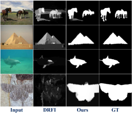
Unlike eye-fixation prediction models, which typically highlight sparse blob-like salient regions, salient object detection models aim to generate smoothly connected areas. A critical step in salient object detection is to distinguish salient objects from their surroundings. To this end, many existing algorithms use intrinsic cues, like uniqueness and surroundedness, to estimate a saliency map for an input image [Perazzi et al., 2012] [Zhang and Sclaroff, 2015]. However, using intrinsic cues alone often produces unsatisfactory results. Therefore, some other models argue that salient objects share common visual attributes, and adopt extrinsic cues to assist in detection. This can be achieved through learning a salient object detector from a set of manually annotated images [Huaizu et al., 2013] [Kim et al., 2014], leveraging statistical features of visually similar images [Singh et al., 2015], or exploiting depth/light field cues [Zhang et al., 2015b]. An overview of salient object detection is presented in [Borji et al., 2014].
In this paper, we offer fresh insights into the application of both intrinsic and extrinsic cues during automatic detection of salient objects. First, our approach involves computation of dense saliency features from within a given image, which involves integration of intrinsic cues. In other words, a vector (SF descriptor) is generated for each pixel of the image to represent its saliency property. This per-pixel SF descriptor is called a "SF image". Second, extrinsic cues derived from ground-truth annotations (or mask) of an example image are used to facilitate the detection of salient objects. To be more specific, using the SF image of an input, the best match is retrieved from references based on its global saliency features (GSF descriptor). Since the existing references are manually annotated, the annotations from the best match (example image) are transferred to the input image to roughly annotate the salient regions. Third, the transferred mask is refined by using objectness proposals, thus creating an initial map. Finally, a coarse-to-fine optimization framework is used in conjunction with the transferred mask and the initial map to produce a high-resolution, full-field saliency map. Overall, the reasonable integration of both intrinsic and extrinsic cues by this method increases the reliability and accuracy of salient object detection, even in particularly challenging images (see Figure 1).
The method outlined in this study is training-free, so it avoids the tedious and time-consuming training task (e.g. it takes over 24h for DRFI [Huaizu et al., 2013] to train a saliency detector). To incorporate extrinsic cues, our approach requires fewer than 20 high-quality references with ground truths, where only a single reference (example image) is needed at a time, from which annotations will be transferred. In addition, this proposed method uses the GSF and SF descriptors designed by ourselves rather than widely used descriptors, such as GIST and SIFT, to find the nearest neighbor and establish dense correspondences. This allows the method prevents scene content from being a limiting factor. Therefore, this method differs substantially from previous methods [Wang et al., 2011][Singh et al., 2015] that need a large collection covering all image categories and visually similar images to provide a discriminant background. Our main contributions are summarized as follows:
- ÷ This paper proposes a new method for salient object detection using both intrinsic (within each testing image) and extrinsic (from an example image) information: (i) Different from other methods using various intrinsic cues to calculate a saliency value, our method integrates them in a new way to represent the saliency property of an image. (ii) We propose a novel GSF descriptor to provide an overall SF image description, which helps us construct references and find one suitable example. (iii) Based on (i) and (ii), we devise a pixel-wise, crosscategory scheme for annotation transfer. Finally, (iv) we design a novel coarse-to-fine optimization framework to optimize the result.
- ÷ The proposed method is compared to a number of topranked salient object detection algorithms on several commonly-used datasets, showing a distinct improvement on the state-of-the-art algorithms.
2 Approach
2.1 Overview
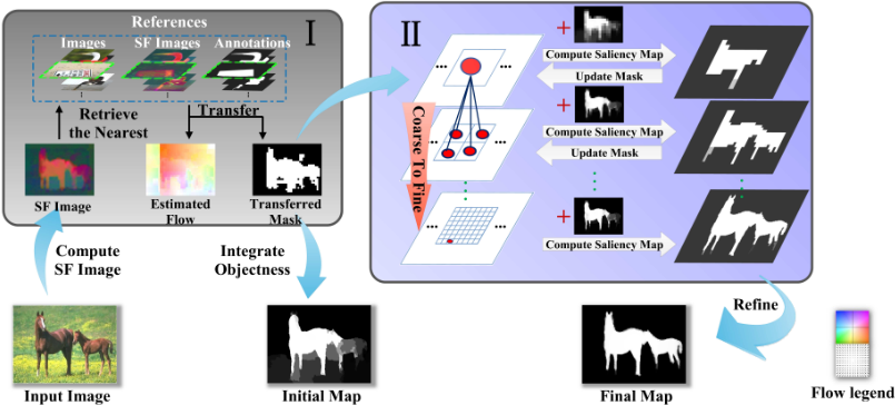
As shown in Figure 2, the method proposed in this study can be divided into two stages. In the first stage, dense low-level saliency features (SF image) are constructed for an input image based on surroundedness cue, boundary prior and convex hull prior. Then, we retrieve the nearest neighbor of the SF image from the references as its example image, and establish dense, pixel-to-pixel correspondences between the input and the example image. During annotation transfer, we warp the manual annotations (or mask) of the example image onto the input image according to estimated dense correspondences, imposing spatial smoothness while preserving discontinuities. By utilizing generic object proposals, the initial map combining both high-level object concepts and lowlevel features is generated.
In the second stage, the accuracy and reliability of the result are increased by using our saliency optimization framework. Firstly, the proposed method computes a more accurate saliency map as a temporary result. Then, the temporary result, along with other information, such as color and location, is used to update the transferred mask, thus increasing the precision of the foreground/background color information for the next layer. The interactions described above iterate at multiple spatial extents from coarse to fine, which reduce running time and guarantee a sufficient number of interactions to produce a high-quality result.
Based on the size of the detected salient object, this method erodes away very small separate areas which are likely background regions, as well as smoothes the edges with the guided filter [He et al., 2013]. This finally results in the accurate, clean and uniform detection of salient objects as displayed in Figure 2.
2.2 SF Image Construction
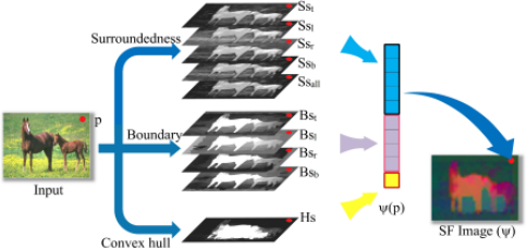
Unlike most existing approaches that directly compute a saliency score or combine independent measures together to finally form a saliency value, our method generates a 10dimensional descriptor that integrates important intrinsic cues for each pixel. Ideally, the descriptor should be able to characterize saliency, and also remain consistent across scenes. To this end, a SF image is constructed based on surroundedness cue, boundary prior and convex hull prior. This assists in the capture of these three properties from a scene, regardless of texture, scale or shape of the visual content of the image.
The Boolean map-based method, which allows effective quantification of the surroundedness property of each region, is used when employing the surroundedness cue. Our method generates a set of Boolean maps B = ¶B1↪B2↪ · · · ↪Bn♦ by evenly thresholding the CIELab color space of an input image. It then constructs attention maps A(B) = ¶A(B)t↪ A(B)l↪ A(B)r↪ A(B)b♦ using the flood fill algorithm to mask out pixels connected to the top, left, right and bottom boundary of the image, respectively. This results in four-fold the number of attention maps as the original BMS [Zhang and Sclaroff, 2015], and thus, when salient objects touch the image edge, more detailed information is recorded with little loss of surroundedness information. To compute the surroundedness property (Ssd) in a certain direction, the following formula is employed:
where d is the direction (e.g. top), and A(B)d denotes the attention map computed by masking out the pixels connected to the boundary in the d direction.
To further distinguish between completely and partially surrounded areas, the complete surroundedness value (Ssall) is computed as using Formula 2:
As is shown in [Yang et al., 2013], the regions along the four boundaries of an image are usually non-salient. Therefore, the boundary prior is used to capture another fundamental property of a scene. Taking the top boundary for an example, we used the SLIC [Achanta et al., 2012] algorithm to oversegment the input image into N small superpixels and treat the superpixels along the top boundary as background seeds for saliency propagation. The result of this propagation is expressed by an N-dimensional vector f ⇤ t , and the top boundary-based saliency Bst, which can be written as in Formula 3:
where i denote a superpixel node.
Similarly, by using the bottom, left, right boundary and the regions outside the convex hull [Xie et al., 2013] as background seeds, we can compute the other three boundarybased saliency properties Bsb, Bsl, Bsr and convex hullbased saliency information Hs.
As shown in Figure 3, these properties are integrated to form a 10-dimensional vector for each pixel p, which is denoted as (p) and computed as follows:
where Ss(p), Bs(p) and Hs(p) denote the computed saliency properties of pixel p based on the surroundedness cue, boundary prior and convex hull prior, respectively.
2.3 GSF Descriptor
In this paper, a novel GSF (global saliency features) descriptor is constructed to summarize the saliency information for different parts of an image, thus providing an overall SF image description. Specifically, the GSF descriptor is computed by dividing each feature layer of a given SF image into twelve sub-regions (a 3⇥4 grid), and then a histogram with ten bins is created for each sub-region. The resulting values from all 10 feature layers are concatenated and a 12⇥10⇥10 = 1200 GSF descriptor is generated. Because this 1200-dimensional descriptor can characterize the global saliency information of an image, it is used to select references and retrieve the nearest neighbor of the input.
Creation of the Reference Set. A key component of our method is a small set of carefully chosen and manually annotated reference images. To this end, 1,000 images are firstly randomly chosen from three publicly available datasets, including MSRA [Liu et al., 2011b], SED [Alpert et al., 2012], and iCoSeg [Batra et al., 2009]. Next, a GSF descriptor is generated for each of these images. Based on their GSF descriptors, we use message-passing based clustering [Frey and Dueck, 2007] to divide them into groups. In each group, the images should share similar global saliency properties. Thus, only two images in each group are selected to represent the different types of SF images, where one is a cluster center and the other is randomly selected. Finally, fewer than 20 images in total are carefully chosen to serve as the reference images.
Retrieval of the Example Image. The objective of example image retrieval is to retrieve the nearest neighbor from the references for the input. Here, we simply use Euclidean distance of GSF to measure the similarities between images, where only the top match is selected each time as the example image. Once the example image is obtained, our next task is to establish the dense, pixel-to-pixel correspondences between the input and example image.
2.4 Annotation Transfer
As our goal is to transfer the annotations from an example image to assist in detection of the salient regions of an input image, it is essential to find the dense saliency correspondence for images across scene contents. Similar to SIFT flow [Liu et al., 2011a], we want SF descriptor to be matched along the flow vector, and the flow field to be smooth, with discontinuities agreeing with object boundaries. Let (p) and 0 (p) be the 10-dimensional saliency vector for the two images at the location of pixel p, respectively. Our task is to estimate the flow vector w(p) = (u(p)↪ v(p)) which preserves both the discontinuous motion field and the spatially coherent information for every pixel. The energy we optimize is a weighted sum of three terms: a data term, a small displacement term and a smoothness term as shown in Formula 5:
where t and d are constant threshold values, and " is the spatial neighborhood of a pixel. Our data term ensures matching by constraining the (p) along with the flow vector w(p). The small displacement term ensures that the flow vectors are as small as possible, while the smoothness term encourages similarity between the flow vectors of adjacent pixels. We minimize this objective function using loopy belief propagation to find the optimal correspondence of each pixel. Finally, the estimated flow w is used to transfer known saliency annotations from the retrieved example to the input image.
Importantly, because the SF image is constructed using low-level saliency concepts, the transferred result may be sensitive to background clutters. To filter out these clutters and other errors, we adopt the method of [Wang et al., 2015] which utilizes high-level objectness to further refine our transferred mask. The refined map, also known as the initial map in this paper, integrates both low-level concepts and high-level objectness. However, at this point, the initial map is still inaccurate and fuzzy (see Figure 2). Therefore, we present a coarse-to-fine saliency optimization framework to generate the clean and high-quality saliency map in the following section.
2.5 Coarse-to-fine Saliency Optimization
To address issues of inaccuracy and uncertainty in the initially generated map, we design a coarse-to-fine saliency optimization framework. Basically, we model salient object detection as an optimization problem for saliency values at multiple spatial extents, ranging from coarse-grid to fine-grid cells. Using multi-level grid sizes, the image is divided into rectangular grid cells, where each grid cell is represented by the mean color of the pixels belonging to and the finest cells are only one pixel in width. Then, we represent the image with a graph, and each grid cell with a node. Edges connect all neighboring nodes of the same level.
We start by computing the more accurate saliency map at the coarsest layer by integrating the transferred mask and the initial map, which provide foreground/background color information and objectness information, respectively. In a similar manner to [Cheng et al., 2015], based on the scaled transferred mask, the foreground probability of node i in the graph is computed as fi = f(φ1↪i) f(φ1↪i)+f(φ0↪i) , where f(φ1↪ i) and f(φ0↪ i) represent the probability of a node i, belonging respectively to the foreground model φ1 and the background model φ0. f(φ1↪ i) and f(φ0↪ i) are computed by using Gaussian Mixture Models (GMMs). Then, the cost function for generating saliency map S is given as follows:
where Si 2 [0↪ 1]. This function contains an initial saliency map term, a foreground/background term and a smoothness term. The initial map term serves as a constraint that ensures that the final saliency value Si is similar to the initial saliency value Ci. The foreground/background term encourages a node with a high foreground probability to be 1 and vice versa. fi and bi denote the foreground and background probability, respectively, where fi + bi = 1. The smoothness term encourages adjacent nodes with similar color to be labeled the same. wij = exp(- dist2 (i↪j) 2σ2w ) represents the weight between two neighboring nodes, where dist(i↪ j) denotes the Euclidean distance between their average colors in the CIELab color space.
Before proceeding to the next layer, the computed saliency map is used to update the transferred maskMusing the cost function displayed in Formula 7:
where Mi= 0 or 1. The first term encourages nodes with a high saliency value to be the foreground, while the second term encourages coherence in nearby nodes with similar color. The updated mask then becomes the input for the next layer so as to provide more precise foreground/background color information.
The interactions described above keep iterating until after calculation of the finest layer is complete. The inaccuracy and uncertainty in the initial map are gradually reduced. Hence, the output of the finest layer is close to perfect. Finally, by eroding very small separate areas and using the guided filter [He et al., 2013] to smooth the edges of the object, we create the final saliency map.
3 Experiments
Implementation. Input images are resized to be 400 ⇥ 300 pixels or 300⇥400 pixels beforehand to ensure that they can be evenly divided by the grids (the coarsest grid is 10 ⇥ 10 pixels). We set ↵ = 0▷0005, β = 1, and d = 40 in Formula 5. We set θ = 0▷3 and ' = 0▷5 in Formula 6. The reference set includes 14 images carefully chosen from three publicly available datasets. These parameters and references are fixed in the following experiments.
Datasets. To evaluate the proposed saliency transfer approach (abbreviated to "STR"), standard benchmark datasets, MSRA1000 [Liu et al., 2011b], ECSSD [Yan et al., 2013], SED1 [Alpert et al., 2012], SED2 [Alpert et al., 2012], SOD [Movahedi and Elder, 2010] and iCoSeg [Batra et al., 2009], are used. MSRA1000, a relatively simple database, has been the most widely used dataset in previous works. The other five databases contain more challenging images. ECSSD includes 1,000 semantically meaningful, but structurally complex images. SED1 and SED2 contain salient objects in a range of sizes and locations. SOD and iCoSeg, the most challenging of the datasets, include images containing multiple salient objects of various sizes at different locations.
Methods of Comparison. The proposed STR is qualitatively and quantitatively compared with several state-of-theart methods and recently published approaches. We first consider the Top 6 salient object detection models ranked by the recent survey [Borji et al., 2015], including DRFI [Huaizu et al., 2013], RBD [Zhu et al., 2014], DSR [Li et al., 2013], MC [Jiang et al., 2013], HDCT [Kim et al., 2014], and HS [Yan et al., 2013]. In addition, we also include five leading methods proposed in 2015: BSCA [Qin et al., 2015], BL [Tong et al., 2015], TLLT [Gong et al., 2015], AH [Van Nguyen and Sepulveda, 2015], and MB+ [Zhang et al., 2015a].
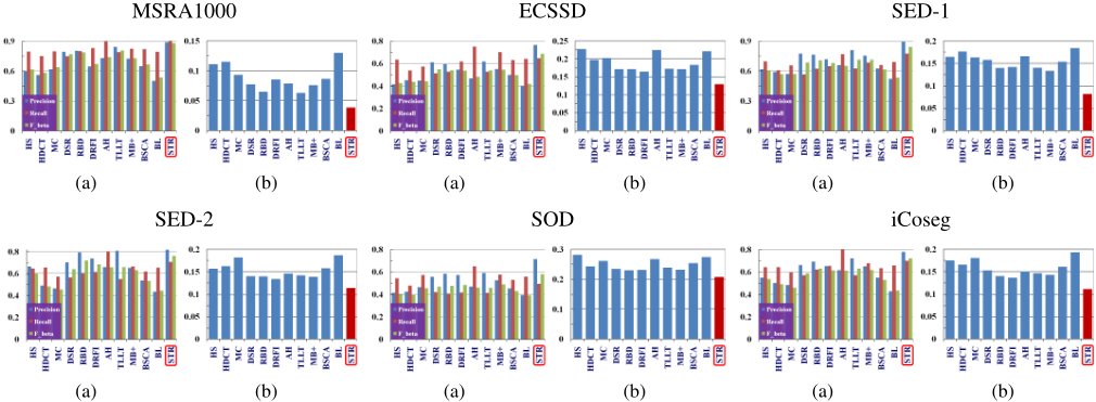
Evaluation Metrics. Previous publications have typically ranked models using metrics like Precision-Recall curve (PR curve), Fβ - measure, and Area Under the Curve (AUC). However, as Margolin et al point out, these traditional metrics may not reliably evaluate the quality of a saliency map due to certain flaws in interpolation, dependency and equal importance [Margolin et al., 2014]. Therefore, a better measure [Margolin et al., 2014], which relies on weighted precision (Precisionw ), weighted recall (Recallw ) and weighted Fβ -measure (F w β ), is adopted to evaluate the performance of the algorithm in this paper. As in [Gong et al., 2015], we set the parameter β2 in F w β = (1+β2 ) Precisionw +Recallw β2P recisionw +Recallw to 0.3 to emphasize the precision. Additionally, we adopt the widely-used mean absolute error (MAE) [Perazzi et al., 2012] which provides a fair estimation of the dissimilarity between the saliency map and ground truth for a more balanced comparison.
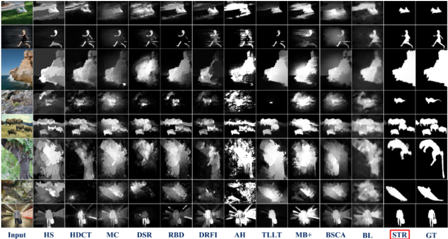
Performance Comparison. In all cases, we use the code or the saliency maps published by the authors of each method. As shown in Figure 4, when detecting salient objects in all six datasets, our method achieves significantly better F w β and MAE scores than all the other methods. Specifically, on MSRA1000, ECSSD, SED1, SED2, SOD and iCoSeg, it respectively improves by 9.17%, 25.16%, 18.05%, 6.15%, 18.80% and 14.40% according to F w β scores, and by 39.05%, 21.22%, 38.83%, 15%, 10.27% and 18.58% in terms of MAE score over the previous best results. As displayed in Figure 5, our method generates cleaner, more reliable and accurate saliency maps than the other methods for a number of different challenges.
| Method | RBD | HS | HDCT | MC | DSR | DRFI | AH | TLLT | MB+ | BSCA | BL | STR |
|---|---|---|---|---|---|---|---|---|---|---|---|---|
| Time(s) | 0.27 | 0.53 | 11.6 | 1.19 | 3.68 | 15.1 | 0.07 | 2.49 | 0.02 | 1.92 | 22.6 | 6.45 |
| Code | Matlab | EXE | Matlab | Matlab | Matlab | Matlab | C++ | Matlab | EXE | Matlab | Matlab | Matlab |
Computational Efficiency. The average running time of each method is tested on a PC with an i5 2.50 GHz CPU and 8GB RAM and the results are listed in Table 1. Our STR is implemented by using MATLAB with unoptimized codes. The method presented in this study takes an average of 6.45 seconds to process an image using a single thread. Although STR is not the fastest method, yet it achieves the best performance (see Figure 4 and 5). We believe that a parallel implementation of our method will largely boost its computational efficiency.
4 Conclusions
In order to address the salient object detection problem, we present a novel method that involves the transfer of annotations from an example image to an input image. The transferred annotations are further refined by integrating high-level objectness. A coarse-to-fine saliency optimization framework is proposed to reliably and efficiently filter out clutters and other errors. Overall, our method achieves satisfactory results on all six challenging benchmarks. In the future, we plan to integrate more cues when constructing SF descriptor and use parallel computing to improve the efficiency of our method.
Acknowledgments
This work was supported in part by the Special Funds of Application-oriented R&D projects (2015B010131002), the University-Industry Cooperation Projects of Guangdong Province (2014A090906004), and the National Natural Science Foundation of China (61370073).
@inproceedings{ijcai2016p482,
  title     = {Saliency Transfer: An Example-Based Method for Salient Object Detection},
  author    = {Li, Xin and Yang, Fan and Chen, Leiting and Cai, Hongbin},
  booktitle = {Proceedings of the Twenty-Fifth International Joint Conference on
               Artificial Intelligence, {IJCAI-16}},
  publisher = {AAAI Press / International Joint Conferences on Artificial Intelligence},
  editor    = {Subbarao Kambhampati},
  pages     = {3411--3416},
  year      = {2016},
  month     = {7},
  url       = {https://ijcai.org/proceedings/2016/482},
}
TY - CPAPER TI - Saliency Transfer: An Example-Based Method for Salient Object Detection AU - Li, Xin AU - Yang, Fan AU - Chen, Leiting AU - Cai, Hongbin T2 - Proceedings of the Twenty-Fifth International Joint Conference on Artificial Intelligence, IJCAI-16 PB - AAAI Press / International Joint Conferences on Artificial Intelligence PY - 2016 SP - 3411 EP - 3416 UR - https://ijcai.org/proceedings/2016/482 ER -Copied
Machine-readable versions of this paper, for tools and AI agents:





