
Visual Tracking with Reliable Memories
Proceedings of the Twenty-Fifth International Joint Conference on Artificial Intelligence. Pages 3491-3496.
Abstract
In this paper, we propose a novel visual tracking framework that intelligently discovers reliable patterns from a wide range of video to resist drift error for long-term tracking tasks. First, we design a Discrete Fourier Transform (DFT) based tracker which is able to exploit a large number of tracked samples while still ensures real-time performance. Second, we propose a clustering method with temporal constraints to explore and memorize consistent patterns from previous frames, named as reliable memories. By virtue of this method, our tracker can utilize uncontaminated information to alleviate drifting issues. Experimental results show that our tracker performs favorably against other state-of-the-art methods on benchmark datasets. Furthermore, it is significantly competent in handling drifts and able to robustly track challenging long videos over 4,000 frames, while most of others lose track at early frames.
- [Avidan, 2007] S. Avidan. Ensemble Tracking. PAMI, 29(2):261, 2007.
- [Babenko et al., 2011] Boris Babenko, Ming-Hsuan Yang, and Serge Belongie. Robust object tracking with online multiple in- stance learning. PAMI, 33(8):1619-1632, 2011.
- [Bolme et al., 2010] David S. Bolme, J. Ross Beveridge, Bruce A. Draper, and Yui Man Lui. Visual object tracking using adaptive correlation filters. In CVPR, pages 2544-2550, 2010.
- [Collins and Liu, 2003] Robert Collins and Yanxi Liu. On-line se- lection of discriminative tracking features. In ICCV, pages 346- 352, 2003.
- [Dalal and Triggs, 2005] Navneet Dalal and Bill Triggs. His- tograms of oriented gradients for human detection. In CVPR, volume 1, pages 886-893, 2005.
- [Danelljan et al., 2014a] Martin Danelljan, Gustav Häger, Fahad Khan, and Michael Felsberg. Accurate scale estimation for ro- bust visual tracking. In British Machine Vision Conference, Not- tingham, September 1-5, 2014. BMVA Press, 2014.
- [Danelljan et al., 2014b] Martin Danelljan, Fahad Shahbaz Khan, Michael Felsberg, and Joost van de Weijer. Adaptive color at- tributes for real-time visual tracking. In CVPR, pages 1090-1097, 2014.
- [Dinh et al., 2011] Thang Ba Dinh, Nam Vo, and Gérard Medioni. Context tracker: Exploring supporters and distracters in uncon- strained environments. In CVPR, pages 1177-1184. IEEE, 2011.
- [Gao et al., 2014] Jin Gao, Haibin Ling, Weiming Hu, and Junliang Xing. Transfer learning based visual tracking with gaussian pro- cesses regression. In ECCV, pages 188-203. Springer, 2014.
- [Girshick, 2015] Ross Girshick. Fast r-cnn. In ICCV, 2015.
- [Grabner et al., 2008] Helmut Grabner, Christian Leistner, and Horst Bischof. Semi-supervised on-line boosting for robust track- ing. In ECCV, pages 234-247. Springer, 2008.
- [Gray, 2005] Robert M Gray. Toeplitz and circulant matrices: A review. Communications and Information Theory, 2(3):155-239, 2005.
- [Hare et al., 2011] Sam Hare, Amir Saffari, and Philip HS Torr. Struck: Structured output tracking with kernels. In ICCV, pages 263-270. IEEE, 2011.
- [He et al., 2015] Kaiming He, Xiangyu Zhang, Shaoqing Ren, and Jian Sun. Spatial pyramid pooling in deep convolutional net- works for visual recognition. Pattern Analysis and Machine In- telligence, IEEE Transactions on, 37(9):1904-1916, 2015.
- [Henriques et al., 2012] João F. Henriques, Rui Caseiro, Pedro Martins, and Jorge Batista. Exploiting the circulant structure of tracking-by-detection with kernels. In ECCV, pages 702-715, 2012.
- [Henriques et al., 2015] J. F. Henriques, R. Caseiro, P. Martins, and J. Batista. High-speed tracking with kernelized correlation filters. PAMI, 2015.
- [Jepson et al., 2003] Allan D Jepson, David J Fleet, and Thomas F El-Maraghi. Robust online appearance models for visual track- ing. PAMI, 25(10):1296-1311, 2003.
- [Jia et al., 2012] Xu Jia, Huchuan Lu, and Ming-Hsuan Yang. Vi- sual tracking via adaptive structural local sparse appearance model. In CVPR, pages 1822-1829. IEEE, 2012.
- [Kalal et al., 2012] Zdenek Kalal, Krystian Mikolajczyk, and Jiri Matas. Tracking-learning-detection. PAMI, 34(7):1409-1422, 2012.
- [Krizhevsky et al., 2012] Alex Krizhevsky, Ilya Sutskever, and Ge- offrey E. Hinton. Imagenet classification with deep convolutional neural networks. In NIPS, pages 1097-1105.
- Curran Associates, Inc., 2012.
- [Kwon and Lee, 2010] Junseok Kwon and Kyoung Mu Lee. Visual tracking decomposition. In CVPR, pages 1269-1276, 2010.
- [Mei and Ling, 2011] Xue Mei and Haibin Ling. Robust visual tracking and vehicle classification via sparse representation. TPAMI, 33(11):2259-2272, 2011.
- [Nummiaro et al., 2003] Katja Nummiaro, Esther Koller-Meier, and Luc Van Gool. An adaptive color-based particle filter. IVC, 21(1):99-110, 2003.
- [Oron et al., 2012] Shaul Oron, Aharon Bar-Hillel, Dan Levi, and Shai Avidan. Locally orderless tracking. In CVPR, pages 1940- 1947. IEEE, 2012.
- [Ren et al., 2015] Shaoqing Ren, Kaiming He, Ross Girshick, and Jian Sun. Faster R-CNN: Towards real-time object detection with region proposal networks. In NIPS, 2015.
- [Rifkin et al., 2003] Ryan Rifkin, Gene Yeo, and Tomaso Poggio. Regularized least-squares classification. Nato Science Series Sub Series III Computer and Systems Sciences, 190:131-154, 2003.
- [Ross et al., 2008] David A Ross, Jongwoo Lim, Ruei-Sung Lin, and Ming-Hsuan Yang. Incremental learning for robust visual tracking. IJCV, 77(1-3):125-141, 2008.
- [Schölkopf et al., 2001] Bernhard Schölkopf, Ralf Herbrich, and Alex J. Smola. A generalized representer theorem. In COLT, pages 416-426, 2001.
- [Viola and Jones, 2001] Paul Viola and Michael Jones. Rapid ob- ject detection using a boosted cascade of simple features. In CVPR, pages I-511, 2001.
- [Wang and Lu, 2014] Dong Wang and Huchuan Lu. Visual tracking via probability continuous outlier model. In CVPR, pages 3478- 3485. IEEE, 2014.
- [Wu et al., 2013] Yi Wu, Jongwoo Lim, and Ming-Hsuan Yang. Online object tracking: A benchmark. In IEEE Conference on Computer Vision and Pattern Recognition (CVPR), 2013.
- [Yilmaz et al., 2006] Alper Yilmaz, Omar Javed, and Mubarak Shah. Object tracking: A survey. ACM Comput. Surv., 38(4), 2006.
- [Zeiler and Fergus, 2014] Matthew D Zeiler and Rob Fergus. Vi- sualizing and understanding convolutional networks. In ECCV, pages 818-833. Springer, 2014.
- [Zhang et al., 2014a] Jianming Zhang, Shugao Ma, and Stan Sclaroff. Meem: Robust tracking via multiple experts using en- tropy minimization. In ECCV, pages 188-203. Springer, 2014.
- [Zhang et al., 2014b] Tianzhu Zhang, Si Liu, Narendra Ahuja, Ming-Hsuan Yang, and Bernard Ghanem. Robust visual track- ing via consistent low-rank sparse learning. IJCV, pages 1-20, 2014.
- [Zhong et al., 2012] Wei Zhong, Huchuan Lu, and Ming-Hsuan Yang. Robust object tracking via sparsity-based collaborative model. In CVPR, pages 1838-1845. IEEE, 2012.
References were extracted automatically from the PDF and may contain errors.
Full text extracted automatically from the PDF; figures, tables and equations may differ. The PDF is the version of record.
1 Introduction
Visual tracking is one of the fundamental and challenging problems in computer vision and artificial intelligence. Though much progress has been achieved in recent years [Yilmaz et al., 2006; Wu et al., 2013], there are still unsolved issues due to its complexity on various factors, such as illumination and angle changes, clutter background, shape deformation and occlusion. Extensive studies on visual tracking employ a tracking-by-detection framework and achieve promising results by extending existing machine learning methods (usually discriminative) with online learning manner [Avidan, 2007; Grabner et al., 2008]. To adaptively model various appearance changes, they deal with a large amount of samples 1 at both detection and updating stages. However, all of them face the same dilemma: While more samples grant better accuracy and adaptiveness, they also come with higher computational cost and risk of drifting. In addition to discriminative methods, [Ross et al., 2008; Mei and Ling, 2011; Wang and Lu, 2014] utilize generative models with a fixed learning-rate to account for target appearance changes. The learning-rate is essentially a trade-off between adaptiveness and stability. However, even with very small rate, former samples' influence on their models still drops exponentially through frames, and drift error may still accumulate. In order to alleviate drift error, [Babenko et al., 2011; Hare et al., 2011; Zhang et al., 2014b] are designed to exploit hidden structured information around the target region. Other methods [Collins and Liu, 2003; Avidan, 2007; Kwon and Lee, 2010] try to avoid drifting by making the current model a combination of the labeled samples in the first frame and the learned samples from the tracking process. However, limited number of samples (e.g., the first frame) can be regarded as "very confident", which in turn restrict their robustness in long-term challenging tasks. Recently, several methods [Bolme et al., 2010; Danelljan et al., 2014b; Henriques et al., 2015] employ Discrete Fourier Transform (DFT) to perform extremely fast detection and achieve high accuracy with the least computational cost. However, same as other generative methods, the memory length of their models is limited by a fixed forgetting rate, and therefore they still suffer from accumulated drift error in long-term tasks.
1 Here "samples" refers to positive (and negative) target patches for trackers based on generative (or discriminative) models.
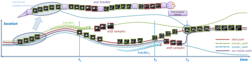
A very important observation is that, when the tracked target moves smoothly, e.g., without severe occlusion or outof-plane rotations, its appearances across frames share high similarity in the feature space (e.g., edge features). Contrarily, when it undergoes drastic movements such as in/out-ofplane rotations or occlusions, its appearances may not be that similar to previous ones. Therefore, if we impose a temporal constraint on clustering these samples, such that only temporally adjacent ones can be grouped together, the big clusters with large intra-cluster correlation can indicate the periods when the target experiences small appearance changes. We take human memory as an analogy for these clusters, using reliable memories to represent large clusters that have been consistently perceived for a long time. In this context, earlier memories supported by more samples have higher probability to be reliable than more recent ones with less support, especially when drift error accumulates across frames. Thus, a tracker may recover from drift error with preference to choose candidates that share high correlation to earlier memories.
Based on these motivations, we propose a novel tracking framework, which efficiently explores self-correlated appearance clusters across frames, and then preserves reliable memories for long-term robust visual tracking. First, we design a DFT-based visual tracker, which is capable of retrieving good memories from a vast number of tracked samples for accurate detection, while still ensures real-time performance. Second, we propose a novel clustering method with temporal constraints to discover distinct and reliable memories from previous frames to help our tracker resist drift error. This method harvests the inherent correlation of the streaming data, and is guaranteed to converge at a fast speed 2 by carefully designing upon Integral Image. To the best of our knowledge, our temporally constrained clustering is novel to vision streaming data analysis, and its high converging speed and promising performance show great potential in online streaming problems. Particularly, it is very competent in discovering clusters (i.e., reliable memories) consisted of uncontaminated sequential samples that are tracked before, and grants our tracker remarkable ability to resist drift error. Experimental results show that our tracker is considerably competent in handling drift error and performs favorably against other state-of-theart methods on benchmark datasets. Further, it can robustly track challenging long videos with over 4000 frames, while most of the others lose track at early frames.
2 Circulant Structure based Visual Tracking
Recent works [Bolme et al., 2010; Henriques et al., 2012; Danelljan et al., 2014b; Henriques et al., 2015] achieve the state-of-the-art tracking accuracy with the least computational cost by exploiting the inherent relationship between DFT and the circulant structure of dense sampling on the target region. In this section, we briefly introduce these methods that are highly related to our work.
Suppose x 2 RL is a vector of an image patch with size M⇥N, centered at the target (L = M⇥N), and xl denotes a
2 Its computational complexity is O(n logn), which costs less than 30 ms for n = 1000 frames.
2D circular shift from x by m⇥n (l is an index for all M⇥N possible shifts, 1 l L). y 2 RL is a vector of a designed response map of size M ⇥ N with a Gaussian pulse centered at the target, too. (x↪ x0 ) =< '(x)↪ '(x0 ) > is a positive definite kernel function defined by mapping '(x) : RL ! RD . We aim to find a linear classifier f(xl) = !T '(xl) + b that minimizes the Regularized Least Square (RLS) cost function:
The first term is an empirical risk to minimize the difference between the designed gaussian response y and the mapping x ! fL(x) 2 RL, where fl(x) = f(xl). The second term ♣♣f♣♣ is a regularization term. It is denoted by ♣♣f♣♣ since it lies in the Kernel Hilbert Space reproduced by .
By Representer Theorem [Sch¨olkopf et al., 2001], cost "(!) can be minimized by a linear combination of inputs: ˆ! = Pl ↵l'(xl). By defining kernel matrix K 2
RL⇥L↪K(l↪ l0 ) = (xl↪ xl0 ), a much simpler form for Eq. 1 can be derived as:
This function is convex and differentiable, and has a closed formminimizer ˆ↵ = (K+λI)-1y. As proved in [Henriques et al., 2012], if the kernel is unitarily invariant, its kernel matrix K is a circulant matrix, that K = C(k), where vector k 2 RL, ki = (x↪ P ix). P i is a permutation matrix that shifts vectors by i-th element(s), C(k) is a circulant matrix from k by concatenating all L possible cyclic shifts of k. and ˆ↵ can be obtained without inverting (K+ λI) by:
where F and F -1 are DFT and its inverse, and is an n by 1 vector with all entries to be 1. Division in Eq. 3
is in Fourier domain, and is thus performed element-wise. In practice, there is no need to compute ˆ↵ from ˆA, since fast detection can be performed on given image patch z by ˆ y = F -1 (F(˜k) ⊙ F( ˆ↵)), where ˜k 2 RL with ˜ kl = (z↪ ˆxl). ˆx is the learned target appearance. Pulse peak in ˆ y shows the target translation in input image z. Detailed derivation is in [Gray, 2005; Rifkin et al., 2003; Henriques et al., 2012].
Though recent methods MOSSE [Bolme et al., 2010], CSK [Henriques et al., 2012] and ACT [Danelljan et al., 2014b], have different configurations of kernel functions and features (e.g., dot product kernel leads to MOSSE, and RBF kernel leads to the latter two), all of them employ a simple linear combination to learn target appearance model ¶ˆxp ↪ ˆAp ♦ at current frame p by
While CSK updates its classifier coefficients ˆAp by Eq. 4 directly, MOSSE and ACT update the numerator ˆApN and denominator ˆApD of coefficients ˆAp separately for stability purpose. The learning-rate γ is a trade-off parameter between long memory and model adaptiveness. After expanding Eq. 4 we obtain:
This shows that, all three methods have an exponentially decreasing pattern of memory: Though the learning-rate γ is usually small, e.g., γ = 0▷1, the impact of a sample ¶xj ↪Aj ♦ at a certain frame j is negligible after 100 frames (γ(1 - γ)100 10-8 ). In other words, these learning-rate based trackers are unable to recourse to samples accurately tracked long before to help resist accumulated drift error.
3 ProposedMethod
Aside from the convolution based visual trackers mentioned above, many other trackers [Jepson et al., 2003; Nummiaro et al., 2003; Ross et al., 2008; Babenko et al., 2011] also update their models ˆQ in similar form as ˆQp = (1-γ) ˆQp-1 +γQp with a learning-rate parameter γ 2 (0↪ 1] and suffers from the drifting problem.
We observe that smooth movements usually offer consistent appearance cues, which can be modelled as reliable memories to recover the tracker from drifting issues caused by drastic appearance change (illustrated in Fig. 1). In this section, we first introduce our novel framework that is capable of handling vast number of samples while still ensures fast detection speed. Then we elaborate the details of intelligently arranging past samples into distinct and reliable clusters that grant our tracker resistance to drift error.
3.1 The Circulant Tracker over Vast Samples
Given new positive sample xp at frame p, we aim to build an adaptive model ¶ˆxp ↪ ˆAp ♦ for fast detection in the coming frame p + 1 with sample image z by
where yp+1 is the response map which shows the estimated translation of the target position, vector ˜kp 2 RL, with its l-th entry ˜kp l := (z↪ ˆxpl ). As we advocated, this model ¶ˆxp ↪ ˆAp ♦ should be built upon vast samples for robustness and adaptiveness. Thus, ˆxp should have the form:
As shown, the adaptive learned appearance ˆxp is a combination of past p samples with concentration on xp of a certain proportion γ. Coefficients ¶βj ♦p-1 j=1 represent the correlation between the current estimated appearance ˆ xp and the past appearances ¶xj ♦p-1 j=1 . A proper choice of ¶βj ♦p-1 j=1 should make the model: 1) adaptive to new appearance changes, and 2) consistent with past appearances to avoid risk of drifting. In this paper, we argue that the set ¶βj ♦p-1 j=1 with preference to previous reliable memories can provide our tracker with considerable robustness to resist drift error. We discuss how to find these reliable memories in Sec. 3.2, and their connections with ¶βj ♦p-1 j=1 are introduced in Sec. 3.3.
Now, we focus on finding a set of classifier coefficients ↵ that fit both the learned appearance ˆxp for consistency and the current appearance xp for adaptiveness. Based on Eq. 1 and Eq. 2, we derive the following cost function to minimize:
where the kernel matrix ˆKp = C(ˆkp ), and vector entry ˆ kp l = (ˆxp ↪ ˆxpl ) (similar for Kp and kp ). γ is a balance factor between the memory consistency and model adaptiveness. By setting the derivative rF p↵ = 0, the accurate solution ˆ↵p will have a very complicated form. We observe that the adaptively learned appearance ˆxp should be very close to the current one xp , since it is a linear combination of close appearances in the past ¶xj ♦p-1 j=1 and the current appearance xp , as shown in Eq. 7. Notice both kernel matrix Kp and ˆKp (and their linear combination with λI) is positive semidefinite. By relaxing Eq. 8 with ˆKp ' (1-γ) ˆKp +γKp ' Kp , we obtain an approximate minimizer ˆ↵p in a very simple form:
δ is an L-dimensional vector in the form δ = [1↪ 0↪ ▷▷▷↪ 0]T, with property that C(δ) = I and F(δ) = ( is an L-dimension vector of ones). Note that in the bracket of F -1 (·), division is performed element-wise.
As long as we find a proper set of coefficients ¶βj ♦p-1 j=1 , we can build up our detection model ¶ˆxp ↪ ˆAp ♦ by Eq. 7 and Eq. 9. In the next frame p+1, fast detection can be performed by Eq. 6 with this learned model.
Distance Matrix and Clustering Result Six temporally constrained clusters with distinct appearances
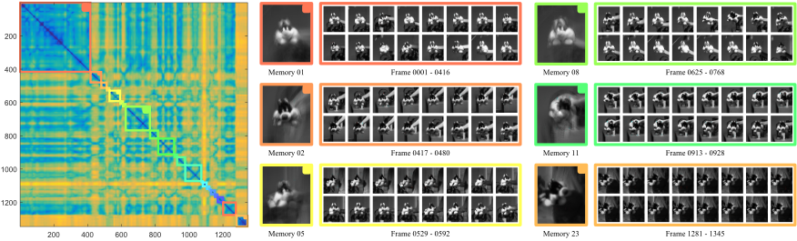
Figure 2: Left: the distance matrix D as described in Alg. 1. Right: Six representative clusters with corresponding colored bounding boxes are shown for intuitive understanding. The image patches in the big bounding boxes is an average appearance of a certain cluster (memory), while the small patches are samples chosen evenly on the temporal domain from each cluster.
Algorithm 1 Temporal Constrained Clustering Algorithm
Input: Integral image J of Distance Matrix D 2 Rp⇥p , s.t. Dij = ♣♣φ(xi ) - φ(xj )♣♣2 ↪ 8i↪ j = 1↪ ▷▷▷↪ p; M= ¶mi♦pi=1 ↪ mi = Piδ↪ 8i = 1↪ ▷▷▷↪ p; Pi is a shifting matrix and δ = [1↪ 0↪ ▷▷▷↪ 0]T; Stoping factor ⇢, and N = ♣M♣ + 1. Output: ˆM= ¶mi♦Hi=1 . while (♣M♣ < N) do N = ♣M♣; for h = 1 : 2 : ♣M♣ do do Evaluate ⌧(sh ↪ sh+1 ) = C(sh T sh+1) - (C(sh ) + C(sh+1 )) using J. if ⌧ (C(sh ↪ sh+1 )) ⇢(C(sh ) + C(sh+1 )) then mh =mh +mh+1, removemh+1 fromM; end if end for end while ˆM = M.3.2 Clustering with Temporal Constraints
In this subsection, we introduce our temporally constrained clustering, which learns distinct and reliable memories from the incoming samples in a very fast manner. Together with the ranked memories (Sec. 3.3), our tracker is robust to inaccurate tracking result, and is able to recover from drift error.
Suppose a set of positive samples are given at frame p: S = ¶xi ♦pi=1 , and we would like to divide them into H subsets ¶sh ♦Hh=1 with indexing vector set M = ¶m1 ↪ ▷▷▷↪mH ♦ 2 ¶0↪ 1♦p , such that sh := ¶xi : mhi = 1↪ 8i = 1↪ ▷▷▷↪ p♦. Our objective are as follows: 1) Samples in each subset sh are highly correlated; 2) Samples from different subsets have relatively large appearance difference, so a linear combination of them is vague or even ambiguous to describe the tracked target (e.g., samples from different viewpoints of the target).
Thus, it can be modeled as a very general clustering problem:
Function C(sh ) measures the average sample distance in feature space φ(·) within subset sh , in the form: C(sh ) = ( p⇥1T ⇥mh )-1 P8xi ↪xj 2sh ↪i<j ♣♣φ(xi ) - φ(xj )♣♣2 . Regularizer r(♣M♣) is a function based on the number of subsets ♣M♣, and ⌘ is a balance factor. This is a discrete optimization problem and known as NP-hard. By fixing the number of subsets ♣M♣ to a certain constant k, k-means clustering can converge to a local optimal.
However, during the process of visual tracking, we do not know the sufficient number of clusters. While too many clusters cause problem of over-fitting, too few clusters may lead to ambiguity. More importantly, as long as we allow random combinations of samples during clustering, any cluster has a risk of taking in contaminated samples with drift error, even wrongly labeled samples, which in turn will degrade the performance of models built upon them.
One important observation is that, target appearances closed to each other in the temporal domain may form a very distinguished and consistent pattern, i.e., reliable memories. E.g,, if a well-tracked target moves around without big rotation or large change in angle for a period of time, its edgebased feature would have much higher similarity compared with feature under different angles. In order to discover these memories, we add temporal constraints on Eq. 10:
Then Eq. 10 with Eq. 11 becomes segmenting S into subsets ¶sh ♦Hh=1 , that each subset only contains timely continuous samples sh = ¶xi ♦vi=u (u↪ v are certain frame numbers).
Still, the constraint of this new problem is discrete and the global optimal can hardly be reached. We carefully designed a greedy algorithm, as shown in Alg. 1, which starts from a trivial status of p subsets. It tries to reduce the regularizer r(♣M♣) in the object function of Eq. 10 by combining temporally adjacent subsets sh and sh+1 , while penalizing the increase of the average sample distance ⌧(sh ↪ sh+1 ) := C(sh T sh+1) - (C(sh ) + C(sh+1 )).
With an intelligent use of Integral Image [Viola and Jones, 2001], the evaluation operation in each combining step in Alg. 1 only takes O(1) running time with integral image J, and each iteration takes linear O(p) operations. The whole algorithm processes in a bottom-up binary tree structure, and runs at O(p log p) in the worst case, and runs less than 30ms on a desktop for over 1000 samples. Designed experiments will show that the proposed algorithm is very competent in finding distinguished appearance clusters (reliable memories) for our tracker to learn.
3.3 TheWorkflow of Our Tracking Framework
Two feature pools are employed in our framework, one for coming positive samples across frames, and the second ( denoted by U) for the learned memories. Every memory u 2 U contains a certain number of samples ¶xuj ♦N u j=1 and a confidence cu:
where N u is the number of samples in memory u and Bu is the beginning frame number of memory u. This memory confidence is consistent with our hypothesis that earlier memories with more samples are more stable and less likely to be affected by accumulated drift error. For each frame, we first detect the object using Eq. 6 to estimate the translation of the target, and then utilize this new sample to update our appearance model ¶ˆxp ↪ ˆAp ♦ by Eq. 7 and Eq. 9.
The correlation coefficient ¶βj ♦p-1 j=1 is then calculated by:
where scalar ⇥ is a normalization term that assures Pp-1 j=1 βj = 1, and ˆu is the most similar memory to the current learned appearance ˆxp in feature space φ(·).
To update memories, we use Alg. 1 to cluster positive samples in the first feature pool into 'memories', and import all except the last one into U. Note when ♣U♣ reaches its threshold, memories with the lowest confidence would be abandoned immediately.
4 Experiments
Our framework is implemented in Matlab with running speed ranges from 12fps to 20fps, on a desktop with an Intel Xeon(R) 3.5GHz CPU, a Tesla K40c video card and 32GB RAM. The adaptiveness ratio γ is empirically set as 0▷15 through all experiments. Stoping factor ⇢ is decided adaptively as 1▷2 times the average covariance of the samples at the first 40 frames on each video. HOG [Dalal and Triggs, 2005] is chosen as the feature φ(·). The maximum number of memories ♣U♣ is set as 10 and max(N u) is set to 100.
4.1 Evaluation of Temporally Constrained Clustering
In order to validate our assumption that temporally constrained clustering on sequentially tracked samples forms reliable and recognizable patterns, we perform Alg. 1 on the off-line positive samples based on our tracking results. Note that our algorithm gives exactly the same result in the online/offline manner, since previously clustered samples have no effect on clustering the unfixed sample afterwards. Due to space limitation, here we present illustrative results from sequences Sylvester in Fig. 2. As shown, the target experiences illumination variation, in-plane and out-of-plane rotation through a long term of 1345 frames. The left part shows the distance matrix D as described in Alg. 1, that Dij = ♣♣φ(xi ) - φ(xj )♣♣2 ↪ 8i↪ j = 1↪ ▷▷▷↪ p. Pixel Dij with dark blue (light yellow) implies small (large) distance between sample xi and xj in feature space φ(·). Different colored diagonal bounding boxes represent different temporally constrained clusters. The right part shows six representative clusters, corresponding to colored bounding boxes on the matrix. Memory #1 and memory #8 are two large clusters containing large amount of samples with high correlated appearance (blue color). Memory #11 represents a cluster with only 16 samples. Its late emergence and limited number of samples result in a very low confidence cu and thus it is not likely to replace any existing reliable memories.
4.2 Boosting by Deep CNN
Our tracker's inherent requirement to efficiently search familiar patterns (memories) at a global scale of the frame overlaps with object detection task [Girshick, 2015; He et al., 2015]. Recently, with the fast development of convolutional neural networks (CNN) [Krizhevsky et al., 2012; Zeiler and Fergus, 2014], Faster-RCNN [Ren et al., 2015] achieves ≥ 5 fps detection speed by using shared convolutional layers for both the object proposal and detection. To equip our tracker with a global vision for its reliable memories, we fine-tune the FC-layers of a Faster-RCNN detector (ZF-Net) once we have learned sufficient memories in a video, which helps our tracker resolve local minimum issues caused by limited effective detection range. Though only supplied with coarse detections with a risk of false alarms, our tracker can start from a local region close to the target and then ensure accurate and smooth tracking results. Note that we only tune the CNN once, with around 150 seconds running time on one Tesla K40c for 3,000 iterations. When the tracking task is long, e.g., more than 3,000 frames, the average fps is larger than 15, which is certainly worthy for significant improvement in robustness. In the following stage, we perform CNN detection every 5 frames, each taking less than 0▷1s.
4.3 Quantitative Evaluation
We first evaluate our method on 50 challenging sequences from OTB-2013 [Wu et al., 2013] against 12 state-of-theart methods: ACT [Nummiaro et al., 2003], ASLA [Jia et al., 2012], CXT [Dinh et al., 2011], DSST [Danelljan et al., 2014a], KCF [Henriques et al., 2015], LOT [Oron et al., 2012], MEEM [Zhang et al., 2014a], SCM [Zhong et al.,

| Sequence / Method | Frame No. | MOSSE | ACT | MEEM | DSST | KCF | DSST (CNN) | KCF (CNN) | TLD | RMT |
|---|---|---|---|---|---|---|---|---|---|---|
| Motocross | 2,035 | 295.9 | 182.5 | 33.4 | 67.5 | 181.5 | 25.2 | 161.2 | 44.7 | 21.5 |
| Volkswagon | 4,000 | 60.6 | 41.3 | 51.1 | 122.7 | 114.1 | 21.3 | 25.3 | 15.9 | 12.3 |
| Carchase | 4,000 | 125.0 | 98.0 | 38.1 | 132.6 | 129.4 | 131.4 | 85.0 | 34.4 | 34.1 |
| Panda | 3,000 | 64.8 | 64.5 | 97.9 | 71.4 | 83.3 | 80.0 | 87.6 | 27.1 | 23.9 |
| Overall | 13,035 | 118.5 | 122.3 | 55.1 | 86.1 | 118.5 | 69.2 | 79.2 | 28.7 | 23.1 |
2012], Struct [Hare et al., 2011], TGPR [Gao et al., 2014], TLD [Kalal et al., 2012] VTD [Kwon and Lee, 2010]. We employed the released code from the public resource (e.g., OTB-2013) or the released version by the authors, and all parameters are fixed for each trackers during testing. Fig. 3 shows the success plots on the whole dataset with the one pass evaluation (OPE) standard. Our tracker, represented as RMT (Reliable Memory Tracker), obtains the best performance, while MEEM, TGPR, KCF and DSST also provide competitive results. It is worth noting that TGPR's idea of building one tracker on auxiliary (very early) samples and MEEM's idea of using tracker's snapshot can be interpreted as making use of early formed memory patterns, which is very relevant to our method. Our tracker outperforms the others on most challenging scenarios, e.g., occlusion, out-of-plane rotation, out of view, fast motion, as illustrated by Fig. 3. The main reason is that our tracker possesses amount of very reliable memories and a global vision that help it regain focus on the target after drastic appearance changes.
In order to explore the robustness of our tracker, and validate its resistance to drift error on long-term challenging tasks, we run our tracker on four long sequences from [Kalal et al., 2012], over 13,000 frames in total. We have also evaluated the convolution filter based methods that are highly related to our method: MOSSE [Bolme et al., 2010], ACT [Nummiaro et al., 2003] and DSST [Danelljan et al., 2014a], KCF [Henriques et al., 2015], together with MEEM [Zhang et al., 2014a] and a detector-based method TLD [Kalal et al., 2012] (shown in Tab. 1). In order to demonstrate the effectiveness of our "reliable memories" in resisting uncontaminated samples for CNN, we also provide the comparison results with the CNN-boosted DSST and KCF. While MOSSE often loses track at very early frames, KCF, ACT and DSST are able to track the target stably for hundreds of frames, but usually cannot maintain their focus after 600 frames. MEEM performs favorably on video Motocross for over 1700 frames with its impressive robustness, but it is unadaptable to scale changes and still leads to inaccurate results. The improvement of KCF and DSST from CNN is still limited, since CNN trained with contaminated samples could lead to inaccuracy (even false alarm), unless these trackers can exclude them from CNN training process as ours do. Our tracker and TLD performs over the other trackers on all videos since both of them have a global vision to search for the target. However, based on an online random forest model, TLD takes in false positive samples slowly, which finally leads to false detections and inaccurate tracking results. Contrarily, guided by the CNN detector trained with our reliable memories, our tracker is only affected by very limited number of false detections. It robustly tracks the target across all frames, and gives accurate target location and target scale until the last frame for all four videos 3 .
5 Conclusion
In this paper, we propose a novel tracking framework, which explores temporally correlated appearance clusters across tracked samples, and then preserves reliable memories for robust visual tracking. A novel clustering method with temporal constraints is carefully designed to help our tracker retrieve good memories from a vast number of samples for accurate detection, while still ensures its real-time performance. Experiment shows that our tracker performs favorably against other state-of-the-art methods, with outstanding ability to recover from drift error in long-term tracking tasks.
3 A video clip with more detailed illustration can be found at https://youtu.be/wtZAGzFDjnM.
@inproceedings{ijcai2016p493,
  title     = {Visual Tracking with Reliable Memories},
  author    = {Wang, Shu and Zhang, Shaoting and Liu, Wei and Metaxas, Dimitris N.},
  booktitle = {Proceedings of the Twenty-Fifth International Joint Conference on
               Artificial Intelligence, {IJCAI-16}},
  publisher = {AAAI Press / International Joint Conferences on Artificial Intelligence},
  editor    = {Subbarao Kambhampati},
  pages     = {3491--3496},
  year      = {2016},
  month     = {7},
  url       = {https://ijcai.org/proceedings/2016/493},
}
TY - CPAPER TI - Visual Tracking with Reliable Memories AU - Wang, Shu AU - Zhang, Shaoting AU - Liu, Wei AU - Metaxas, Dimitris N. T2 - Proceedings of the Twenty-Fifth International Joint Conference on Artificial Intelligence, IJCAI-16 PB - AAAI Press / International Joint Conferences on Artificial Intelligence PY - 2016 SP - 3491 EP - 3496 UR - https://ijcai.org/proceedings/2016/493 ER -Copied
Machine-readable versions of this paper, for tools and AI agents:





