
Solving M-Modes Using Heuristic Search
Proceedings of the Twenty-Fifth International Joint Conference on Artificial Intelligence. Pages 3584-3589.
Abstract
M-Modes for graphical models is the problem of finding top M label configurations of highest probability in their local neighborhoods. The state-of-the-art method for solving M-Modes is a dynamic programming algorithm which computes global modes by first computing local modes of each subgraph and then search through all their consistent combinations. A drawback of the algorithm is that most of its time is wasted on computing local modes that are never used in global modes. This paper introduces new algorithms that directly search the space of consistent local modes in finding the global modes, which is enabled by a novel search operator designed to search a subgraph of variables at each time. As a result, the search algorithms only need to generate and verify a small number of local modes and can hence lead to significant improvement in efficiency and scalability.
- [Bach and Jordan, 2003] Francis R Bach and Michael I Jor- dan. Beyond independent components: trees and clusters. JMLR, 4:1205-1233, 2003.
- [Batra et al., 2012] Dhruv Batra, Payman Yadollahpour, Ab- ner Guzman-Rivera, and Gregory Shakhnarovich. Di- verse M-best solutions in markov random fields. Computer Vision-ECCV 2012, pages 1-16, 2012.
- [Biswal et al., 2010] Bharat B Biswal, Maarten Mennes, Xi- Nian Zuo, Suril Gohel, Clare Kelly, Steve M Smith, Chris- tian F Beckmann, Jonathan S Adelstein, Randy L Buckner, Stan Colcombe, et al. Toward discovery science of human brain function. Proceedings of the National Academy of Sciences, 107(10):4734-4739, 2010.
- [Chen et al., 2013] Chao Chen, Vladimir Kolmogorov, Yan Zhu, Dimitris Metaxas, and Christoph H Lampert. Com- puting the M most probable modes of a graphical model. In International Conf. on Artificial Intelligence and Statis- tics (AISTATS), 2013.
- [Chen et al., 2014] Chao Chen, Han Liu, Dimitris Metaxas, and Tianqi Zhao. Mode estimation for high dimensional discrete tree graphical models. In Advances in neural in- formation processing systems, pages 1323-1331, 2014.
- [Chow and Liu, 1968] C Chow and C Liu. Approximating discrete probability distributions with dependence trees. Information Theory, IEEE Transactions on, 14(3):462- 467, 1968.
- [Dechter et al., 2012] Rina Dechter, Natalia Flerova, and Radu Marinescu. Search algorithms for m best solutions for graphical models. In Jrg Hoffmann and Bart Selman, editors, AAAI. AAAI Press, 2012.
- [Eloyan et al., 2012] Ani Eloyan, John Muschelli, Mary Beth Nebel, Han Liu, Fang Han, Tuo Zhao, Anita D Barber, Suresh Joel, James J Pekar, Stewart H Mostofsky, et al. Automated diagnoses of attention deficit hyperactive disorder using magnetic resonance imaging. Frontiers in systems neuroscience, 6, 2012.
- [Fromer and Globerson, 2009] Menachem Fromer and Amir Globerson. An LP view of the M-best MAP prob- lem. Advances in Neural Information Processing Systems, 22:567-575, 2009.
- [Fromer and Yanover, 2009] M. Fromer and C. Yanover. Ac- curate prediction for atomic-level protein design and its application in diversifying the near-optimal sequence space. Proteins: Structure, Function, and Bioinformatics, 75(3):682-705, 2009.
- [Korf et al., 2005] Richard E. Korf, Weixiong Zhang, Igna- cio Thayer, and Heath Hohwald. Frontier search. J. ACM, 52(5):715-748, 2005.
- [Kwisthout, 2008] Johan Kwisthout. Complexity results for enumerating mpe and partial map. In European Workshop on Probabilistic Graphical Models, 2008.
- [Lampert, 2011] C.H. Lampert. Maximum margin multi- label structured prediction. NIPS, 2011.
- [Lichman, 2013] M. Lichman. UCI machine learning repos- itory, 2013.
- [Liu et al., 2011] Han Liu, Min Xu, Haijie Gu, Anupam Gupta, John Lafferty, and Larry Wasserman. Forest den- sity estimation. Journal of Machine Learning Research, 12:907-951, 2011.
- [Marinescu and Dechter, 2009] Radu Marinescu and Rina Dechter. AND/OR branch-and-bound search for combi- natorial optimization in graphical models. Artif. Intell., 173(16-17):1457-1491, 2009.
- [Nilsson, 1998] D. Nilsson. An efficient algorithm for find- ing the m most probable configurationsin probabilistic ex- pert systems. Statistics and Computing, 8(2):159-173, 1998.
- [Nowozin and Lampert, 2010] S. Nowozin and C.H. Lam- pert. Structured learning and prediction in computer vi- sion. Foundations and Trends in Computer Graphics and Vision, 6(3-4):185-365, 2010.
- [Park and Darwiche, 2003] James D. Park and Adnan Dar- wiche. Solving map exactly using systematic search. In Proceedings of the 19th Annual Conference on Uncer- tainty in Artificial Intelligence (UAI-03), pages 459-468, 2003.
- [Pearl, 1988] J. Pearl. Probabilistic Reasoning in Intelligent Systems: Networks of Plausible Inference. Morgan Kauf- mann Publishers, Inc., San Mateo, CA, 1988.
- [Prasad et al., 2014] Adarsh Prasad, Stefanie Jegelka, and Dhruv Batra. Submodular meets structured: Finding di- verse subsets in exponentially-large structured item sets. In Advances in Neural Information Processing Systems, pages 2645-2653, 2014.
- [Wainwright and Jordan, 2008] Martin J Wainwright and Michael I Jordan. Graphical models, exponential fami- lies, and variational inference. Foundations and Trends in Machine Learning, 1(1-2):1-305, 2008.
- [Yadollahpour et al., 2013] Payman Yadollahpour, Dhruv Batra, and Gregory Shakhnarovich. Discriminative re- ranking of diverse segmentations. Proc. of IEEE Confer- ence on CVPR, 2013.
- [Yanover and Weiss, 2004] C. Yanover and Y. Weiss. Find- ing the M most probable configurations using loopy belief propagation. In Advances in Neural Information Process- ing Systems, 2004.
- [Yuan and Hansen, 2009] Changhe Yuan and Eric A. Hansen. Efficient computation of jointree bounds for sys- tematic MAP search. In Proceedings of 21st International Joint Conference on Artificial Intelligence (IJCAI-09), pages 1982-1989, Pasadena, CA, 2009. IJCAI
- [Yuan and Lu, 2007] Changhe Yuan and Tsai-Ching Lu. Finding explanations in Bayesian networks. In Proceed- ings of the 18th International Workshop on Principles of Diagnosis (DX-07), pages 414-419, 2007.
- [Yuan et al., 2011] Changhe Yuan, Heejin Lim, and Tsai- Ching Lu. Most relevant explanation in Bayesian net- works. J. Artif. Intell. Res., 42:309-352, 2011.
References were extracted automatically from the PDF and may contain errors.
Full text extracted automatically from the PDF; figures, tables and equations may differ. The PDF is the version of record.
1 Introduction
In many structured prediction applications, our model is far from perfect. Therefore, it is difficult to trust the single best prediction from the model. In recent years, new methods have been proposed to generate a set of predictions, containing at least one solution that is close to the truth. Such solution set can be fed to other more expensive models [Yadollahpour et al., 2013] or can be used as equally valid hypotheses [Fromer and Yanover, 2009]. The classic M-Best methods [Dechter et al., 2012; Nilsson, 1998; Yanover and Weiss, 2004; Fromer and Globerson, 2009] compute the M most probable predictions, which tend to be very similar to each other. These similar solutions are likely to succeed or fail concurrently, and thus cannot serve the purpose. Recent methods [Lampert, 2011; Batra et al., 2012; Prasad et al., 2014] compute a solution set with not only high probability but also high diversity.
Chen et al. [2013; 2014] proposed to compute top modes, i.e., local maxima, of a graphical model as a high quality solution set. In a discrete domain, a mode is defined as an element with higher probability than all its neighbors. The neighborhood is defined as the ball centered at the element of interest with a radius δ. The top M probable modes provide a global description of the probability landscape, and is a principled solution for generating multiple diverse predictions.
Solving M-Modes is much more challenging than M-Best. To solve the latter problem, we only need to globally compare the probability of different label configurations. For M-Modes, however, a solution should not only have a high probability but also be the mode in its local neighborhood. It is shown that a label configuration is a global mode if and only if it is a local mode in every connected subgraph of size δ [Chen et al., 2013; 2014]. Based on this local-global property, a dynamic programming algorithm has been developed to solve M-Modes by first computing all local models of each subgraph and then searching through all their consistent combinations. The drawback of the DP algorithm, however, is that most of its time is wasted on computing local modes that are never used in the global modes.
In this work, we propose to apply heuristic search to solve M-Modes. Our search algorithms also build on the localglobal property, but directly search for global modes by incrementally piecing together consistent local modes. Such search is enabled by a novel search operator designed to search the local modes of a subgraph of variables at each step. The local modes are not computed a priori, but are generated and verified on the fly. A global mode is found once a consistent combination of local modes of all subgraphs has been identified. Our design of the search steps is quite different from existing search methods for solving various inference problems in graphical models such as MPE [Marinescu and Dechter, 2009; Kwisthout, 2008], MAP [Park and Darwiche, 2003; Yuan and Hansen, 2009], and MRE [Yuan et al., 2011; Yuan and Lu, 2007]. All those algorithms use variables as the basic search units, i.e., they search one variable at a time. In comparison to the DP algorithm, our search algorithm only needs to verify a small number of local modes and can hence lead to significant improvement in efficiency. Empirical results show that the search algorithm indeed is much more efficient and scalable.
2 Background
We focus on undirected graphical models (Markov random fields), although the definitions and algorithms can be easily extended to directed models (Bayesian networks [Pearl, 1988]). A Markov random field (MRF) [Wainwright and Jordan, 2008; Nowozin and Lampert, 2010] models a joint discrete distribution using a graph G = (V↪ E) and a potential function f . The set of vertices/nodes V corresponds to the set of discrete variables i 2 ¶1↪ ▷ ▷ ▷ ↪ d♦, where d = ♣V♣. A node i can be assigned a label xi 2 L. A label configuration of all variables x = (x1↪ ▷ ▷ ▷ ↪ xd) is called a labeling. We denote by X = Ld the domain of all labelings. The potential function f : X ! R assigns to each labeling a real value, which is inversely proportional to the logarithm of the probability distribution, p(x) = exp(-f(x) - A), where A = log Px2X exp(-f(x)) is the log-partition function. Assuming these variables satisfy the Markov properties, the potential function can be written as f(x) = P(i↪j)2E fi↪j(xi↪ xj), where fi↪j : L⇥L!R is the potential function for edge (i↪ j)1 . For convenience, we assume any two different labelings have different potential function values.
We define the following notations for convenience. A vertex subset, V 0 ✓ V, induces a subgraph consisting of V 0 and all edges whose both ends are within V 0 . In this paper, all subgraphs are vertex-induced. Therefore, we abuse the notation and denote both the subgraph and the vertex subset by the same symbol. We call a labeling of a subgraph B a partial labeling. For a given labeling x, we may denote by xB its label configurations of vertices of B. We denote by fB(xB) the potential of the partial labeling, which is only evaluated over edges within B. When the context is clear, we drop the subscript B and write f(xB).
3 M-Modes
In this section, we introduce the problem of M-Modes and review previous solutions. Denote by ⇢(·↪ ·) : X ⇥X ! R the Hamming distance metric on the space of labelings, i.e., the number of variables at which two labelings disagree. Given a scale parameter δ, we define the δ-modes as follows.
Definition 1 (δ-modes). The δ-neighborhood of a point x, Nδ(x), is the ball centered at x with radius δ, formally, ¶y ♣ ⇢(x↪ y) δ♦. A point is a δ-mode if and only if its probability density value is higher than all other elements in Nδ(x).
Modes of different scales provide a multiscale description of the underlying probability landscape. As δ increases, the δneighborhood of each x grows, and the set of δ-modes monotonically shrink until only the global optimum (MAP) is left. We address the main computational problem.
Problem 1 (M-Modes). For a given δ, compute the M δmodes with the highest probability (lowest potential).
Modes are closely related to modes of subgraphs, i.e., local modes conditioned on the labels of surrounding vertices. Given a subgraph B, denote by @B its boundary, i.e., the set of vertices that are adjacent to vertices of B. Denote by ¯B the closure of B, i.e., the disjoint union of B and its boundary.
Definition 2 (local modes). A partial labeling, x ¯B, is a local mode if and only if there is no other partial labeling y ¯B with the same labeling on the boundary (y@B = x@B), has a smaller potential (f(y ¯B) < f(x ¯B)), and is within δ distance from x ¯B (⇢(y ¯B↪ x ¯B) δ).
1 For convenience, we drop unary potentials fi, as they can be absorbed into binary potentials. That is, any potential function with unary potentials can be rewritten as one without them.
Given a graph G and a collection of its subgraphs B = ¶B1↪ B2↪ ▷ ▷ ▷♦, it was shown that under certain condition, there is a close connection between the modes of G and the local modes of closures of these subgraphs, ¯Bi's. In particular, any consistent combinations of these local modes is a global mode, and vice versa [Chen et al., 2014].
Theorem 1 (local-global). Suppose any connected subgraph G0 ✓ G of size δ is contained within some Bi 2 B. A labeling x of G is a global mode if and only if for every ¯Bi, the corresponding partial labeling x ¯Bi is a local mode.
We say partial labelings of two different subgraphs are consistent if they agree at all common vertices. Theorem 1 shows that there is a bijection between the set of global modes and the set of consistent combinations of local modes. This leads to efficient methods for modes computation. It will also be the basis of the search algorithm proposed in this paper.
Chen et al. [2013; 2014] proposed to compute global modes for tree models by first computing all local modes and then searching through all their consistent combinations to find the top M ones. The subgraphs they considered are the set of geodesic balls of radius bδ◁2c centered at all vertices. A junction tree model was constructed whose nodes correspond to these subgraphs. Finding the top M combinations of local modes is equivalent to finding the top M labelings of this junction tree, and can be solved efficiently using dynamicprogramming-based algorithm [Nilsson, 1998]. The computational bottleneck, however, is the computation of the local modes for all geodesic balls. The number of local modes can be very large for each subgraph.
4 Heuristic Search for SolvingM-Modes
In this section, we apply heuristic search to solve the MModes problem. The goal is to utilize the local-global property of modes in Theorem 1 to directly search in the space of consistent local modes in finding global modes. Each step of our algorithm is designed to search a subgraph of variables. We first define the concept of δ-subgraph.
Definition 3 (δ-subgraph). A δ-subgraph of a graphical model is a connected subgraph with size δ. The variables B contained in the subgraph are called interior variables. The adjacent variables @B of B are called boundary variables.
From the definition, we can conclude the following.
Theorem 2. Given a labeling of the boundary variables @B, the local mode over B is also a δ-mode. In fact, the local mode must be the MAP solution over B conditioned on the labeling of @B.
For any δ-subgraph B, different labelings of the boundary variables @B lead to different probability landscapes over B. By definition, the MAP solution over B must be the local mode. A δ-mode must consist of consistent local modes of all possible δ-subgraphs according to the local-global property.
With the key concepts defined, we now introduce two heuristic search algorithms to solve M-Modes. The outline of both algorithms is as follows. First, we create an ordering of all possible δ-subgraphs of a graphical model. Then, we apply depth-first branch and bound (DFBnB) and A* to search for consistent local modes of the δ-subgraphs using the ordering. The local modes are generated and verified when they are needed. An admissible heuristic function is used to evaluate the promisingness of a search node. The algorithms terminate when either the whole search space is explored (DFBnB) or top M solutions have been found (A*). The following subsections explain the details.
4.1 Compiling Ordering of Subgraphs
Our search algorithms need to explore all δ-subgraphs of a graphical model during the search. Depending on the structure of the graphical model, a δ-subgraph may have a chain, tree, or graph structure. We use a preprocessing step to create an ordering of all δ-subgraphs. First, a complete ordering of the variables is created using a topological traversal of the model. Then, for each variable X in the list, we recursively find all δ-subgraphs that are rooted at X. Algorithm 1 provides a pseudo code for this preprocessing step.
Input: G - a graphical model; δ - subgraph size Output: SubGraphs - an ordered list of δ-subgraphs 1: function COMPILESUBGRAPHS(G, δ) 2: SubGraphs ; 3: topo-order TopoOrder(G) 4: for all vertex 2 topo-order do 5: Stack ¶vertex♦ 6: if vertex.degree > 1 then 7: RECURSION(SubGraphs, Stack, δ-1) 8: return SubGraphs 9: function RECURSION(SubGraphs, Stack, budget) 10: if budget > 1 then 11: for all vertex 2 Stack do 12: for all child 2 vertex.Children do 13: if child.topo-order > ¶8 vertex 2 Stack♦. 14: topo-order & child.degree>1 then 15: Stack.push(child) 16: RECURSION(SubGraphs,Stack, 17: budget-1) 18: Stack.pop() 19: else 20: Stack.add(Boundary(Stack)) 21: SubGraphs.push(Stack)Figure 1 shows an example graphical model. Suppose the topological traversal order of the variables is ¶1↪ 2↪ 3↪ 4↪ 5↪ 6♦. If δ is set to be 3, an ordering of all δ-subgraphs is ¶1↪ 2↪ 3♦, ¶1↪ 2↪ 4♦, ¶1↪ 2↪ 6♦, ¶2↪ 3↪ 4♦, ¶2↪ 3↪ 6♦, ¶2↪ 4↪ 5♦, ¶2↪ 4↪ 6♦. It is easy to identify the boundary variables for each δ-subgraph. For example, the shaded variables ¶4↪ 6♦ in Figure 1 are the boundary variables of ¶1↪ 2↪ 3♦.
4.2 Search Algorithms
Now we introduce the algorithms for solving M-Modes, depth-first branch and bound (DFBnB) and A*. We first explain the DFBnB algorithm in detail. Then we will briefly explain howA* works differently.
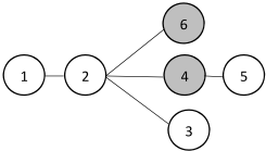
The DFBnB algorithm uses a top list to keep track of the best solutions, and a stack to keep track of search nodes in the current search path. The top list is initialized with M random modes found by a simple hill climbing search. The stack is initialized with search nodes corresponding to different local modes of the first δ-subgraph. Consider the example model, the first δ-subgraph is ¶1↪ 2↪ 3♦. We first enumerate all labelings of its boundary variables ¶4↪ 6♦. Conditioned on each labeling, we calculate the local mode for ¶1↪ 2↪ 3♦, which can be solved using any MAP algorithm. A search node is created for each such local mode plus its boundary labeling. These nodes are pushed to the stack in an increasing order of quality estimated by a heuristic function. The function INITIALEXPAND in Algorithm 2 explains this step.
Then at each iteration, the search algorithm pops out the top node in the stack. Let x stands for the (partial) labeling of all interior and boundary variables of the δ-subgraphs that have been searched so far. If the last δ-subgraph in the ordering has been searched, x must be a global mode. It is added to the top list if the potential of x is higher than that of the worst incumbent solution; the worst solution is then discarded. Otherwise, the top node is discarded.
If the top node is not yet a mode, it is compared to the worst incumbent solution in the top list. If its heuristic estimate is worse than the incumbent, the node is discarded immediately because it will not lead to any better solutions. Otherwise, we generate its successor nodes by searching the next δ-subgraph. Adjacent δ-subgraphs typically have overlaps. Again consider the example, ¶1↪ 2↪ 4♦ is the next δ-subgraph. All variables in ¶1↪ 2↪ 4♦ are either interior or boundary variables of ¶1↪ 2↪ 3♦. So are its boundary variables ¶3↪ 6♦ except one new variable 5. The way we generate the δ-subgraphs makes sure that all interior variables of the current δ-subgraph B must have appeared in earlier δ-subgraphs or their boundaries, so xB is known. But there are two possibilities for the boundary variables @B: (1) there are one or more new boundary variables, denoted as N, or (2) no new variable. In the first case, conditioned on each partial labeling of N and x@B∩N, we need to verify whether xB is a local mode. In the example, all of ¶1↪ 2↪ 4♦ inherit values from x; so are boundary variables ¶1↪ 6♦. We only need to verify, conditioned on each possible value of 5 and x¶1↪6♦, whether x¶1↪2↪4♦ is a local mode. If yes, a successor search node is generated. Otherwise, the search path is discarded because it cannot lead to a consistent global mode. All successors are added to the stack in increasing order of quality.
In the second case with no new boundary variables, the current δ-subgraph B and its boundary variables @B must have appeared in earlier subgraphs. We do not have to perform any search here, but just need to verify whether xB is a local mode conditioned on x@B. This is necessary due to the local-global property of modes. If yes, the current node is put back into the stack and will be selected in the next iteration for searching the next δ-subgraph. If not, the node is discarded. The depth first search algorithm repeats the above search step until the whole search space is explored. Algorithm 2 shows a pseudo code of the DFBnB algorithm.
The A* algorithm works a bit differently. It uses an open list to keep track of unexpanded search nodes. The open list is initialized in a similar way as the stack in DFBnB. At each step, the A* algorithm pops out the best search node in the open list. If the node is a mode, a new solution is found. If not, the successors of the node are generated similarly as in DFBnB and put in the open list. A* repeats the search step until the first M solutions are found, which are guaranteed to be the top Mmodes. Note that the search space is a tree due to the way we search the δ-graphs. The A* algorithm thus does not need a closed list to store expanded nodes and reduces to a frontier A* algorithm [Korf et al., 2005].
4.3 Heuristic Function
This section answers the question on how to estimate the quality of a search node. A search node is evaluated in two parts: the potential of the partial labeling of the δ-subgraphs that have been instantiated, and an estimated potential for the remaining δ-subgraphs. The second part is calculated by a heuristic function. The sum of these two provides a global estimate on the quality of solutions that can be found via the current search path. If the heuristic function provides upper bound estimations, the function is called admissible, which guarantees the optimality of the search algorithms.
For M-Modes, we are searching for the top M labelings with highest potential. All extensions of a search node can be bounded by the potential of the MAP solution over the remaining variables conditioned on the current path represented by the node. We therefore use MAP as the heuristic function. We do not have to do MAP inference for each search node, however. In fact, we only need to perform once the maxproduct MAP algorithm [Wainwright and Jordan, 2008] in the direction opposite to the search order. This backward message propagation is able to provide a probability table for all MAP solutions conditioned on various forward search states. During the search, we only need to look up the table for the heuristic estimate for a search node. This ensures the efficiency of the search algorithm.
5 Empirical Results
We evaluated our method by comparing to the algorithm by Chen et al. [2014] (called DP) on both synthetic and real datasets. Although our search algorithms are applicable to general graphical models, the DP algorithm is limited to treestructured models. To make comparisons possible, we first focused on tree models. We compared the running time of the methods on tree-models with different sizes (d) and tree degrees (t). We also compared the methods with different scales Algorithm 2 Depth-First Branch and Bound Algorithm for Solving M-Modes
Input: G - a graphical model; δ - neighborhood size; M - number of top Labelings Output: TopList - top MLabelings 1: function DFBNB(G, δ, M) 2: Stack ; 3: TopList HCSearch(M) 4: SubGraphs CompileSubGraphs(G, δ) 5: INITIAL-EXPAND(Stack, SubGraphs) 6: while !Stack.isEmpty() do 7: current Stack.pop() 8: if current.g>TopList.last.g then 9: if current.index==SubGraphs.size then 10: TopList.push(current) 11: TopList.removelast() 12: else 13: EXPAND(Stack,current,SubGraphs) 14: return TopList 15: function INITIAL-EXPAND(Stack,SubGraphs) 16: Boundaries Boundary(SubGraphs.first) 17: LocalList ; 18: for all labeling of Boundaries do 19: newstate ; 20: newstate.g δ-Mode(labeling) 21: newstate.path labeling 22: newstate.h MAP(newstate.path) 23: newstate.f newstate.g + newstate.h 24: newstate.index 1 25: LocalList.push(newstate) 26: LocalList.sort() 27: Stack.push(LocalList) 28: function EXPAND(Stack,current,SubGraphs) 29: newIndex current.index + 1 30: newBoundary NewBoundary(SubGraphs. 31: Next(current), current.path) 32: if IsEmpty(newBoundary) then 33: newstate current 34: if IsLocalMode(newstate) then 35: newstate.index newIndex 36: Stack.push(newstate) 37: return 38: LocalList ; 39: for all labeling of newBoundary do 40: newstate current 41: newstate.path.push(labeling) 42: if IsLocalMode(newstate) then 43: newstate.g current.g+ 44: Pvertex2newBoundary vertex▷potential 45: newstate.h MAP(newstate.path) 46: newstate.f newstate.g + newstate.h 47: newstate.index newIndex 48: LocalList.push(newstate) 49: LocalList.sort() 50: Stack.push(LocalList)

(δ) and number of modes to produce (M). The performance on loopy models is reported in the end.
Synthetic Data
We randomly generated tree models with different parameter settings. For each setting, we generated ten tree models and computed the average running time. The label size L was fixed to be three. This experiment is designed to systematically test the influence of each parameter on the search and DP algorithms. However, testing all four parameters at the same time is difficult. Instead, each time we fixed three parameters and varied the remaining parameter. The base setting is d = 60↪ t = 6↪ δ = 3, and M = 4. The results are reported in Figure 2.
The two left figures show that A* and DFBnB were not affected much by dimension and tree degree, while DP slowed down as the parameters increased. It may seem surprising that A* and DFBnB are not affected much by the parameters. The explanation is that the size of the search space is mostly decided by the number of subgraphs. Dimension and tree degrees do not directly affect the number of subgraphs. DP slowed down when the dimension and tree degree increased because the algorithm computes all local modes before running dynamic programming. The expense for computing local modes is high, especially near variables with high degrees.
The two right figures show that A* and DFBnB were significantly affected by δ and M, but DP were not. As δ or M increased to larger values, the running time of A* and DFBnB both increased dramatically. However, the running time started decreasing when δ was around 8. The reason is when δ was relatively small, larger δ increased the number of subgraphs, which in turns made the search space larger. However, as δ kept increasing, the number of subgraphs decreased due to fewer combinations. DFBnB was affected by the increase in M more than A* in this experiment. The speed of DP was invariant to M as the bottleneck is the computation of all local modes. Once these local modes are computed, using DP to compute top M solutions is very efficient and is not slowing down much as we increases M. In the first step, the algorithm computes local modes in an inductive manner; local models of scale δ are computed using local modes of scale δ - 1. Most of the time is spent on δ = 1 case, in which the local modes are computed using enumeration. Therefore, the algorithm does not slow down much as we increase δ. That is also why both A* and DFBnB became slower than DP in face of large δ and M. However, small to medium δ and M are more reasonable choices in real applications. When δ is large, the modes are very sparse. When M is large, we may include many weak modes.
Real Data
We applied our method to tree modes estimated from real world data. We selected data of different dimensions from UCI repository [Lichman, 2013]. These data are categorical, i.e., have discrete values are each dimension. We also used the ADHD-200 dataset [Biswal et al., 2010]. The fMRI data is preprocessed and reduced to 264 dimensions following [Eloyan et al., 2012]. We discretized the continuous feature values into three labels, corresponding to low, normal and high response. We estimated a tree-structured graphical model for each data, using the algorithm by Chow and Liu [1968]. The tree size is equal to the number of dimensions of the feature space. The tree structure is reconstructed by computing a maximum spanning tree of a complete graph in which each edge weight is the empirical mutual information between the corresponding pair of variables. Once the tree structure is determined. The pairwise potentials of each edge are determined using the empirical unary and binary marginals ˆ p (see [Bach and Jordan, 2003; Liu et al., 2011] for more details).
| congress | mushroom | soybean | M.P. | M.S.J. | ADHD | |
|---|---|---|---|---|---|---|
| DFBnB | 0.0230 | 0.3167 | 0.0719 | 0.5888 | 0.0011 | 0.2194 |
| A* | 0.0304 | 0.8886 | 0.0619 | 2.4667 | 0.0011 | 0.0145 |
| DP | 0.1122 | 1.1734 | 1.6723 | 5.0968 | 0.2005 | 6.6018 |
| d | 16 | 22 | 35 | 57 | 60 | 264 |
| t | 6 | 5 | 8 | 6 | 3 | 6 |
Figure 4 shows that DFBnB and A* were both significantly faster than DP. The speedup ranged from several times to several hundred times faster. However, we did not see a clear winner between DFBnB and A*; DFBnB was faster than A* on four datasets, while A* was faster on the remaining three. To gain more insight, we did two more experiments using the mushroom dataset studying the effect of the parameters: (1) fix M = 8 and vary δ, and (2) fix δ = 4 and vary M. The two left figures in Figure 3 show running time (seconds) and peak number of memory units (nodes) for experiment (1), and the two right figures for experiment (2). The left-most figure shows that the running time of DFBnB and A* both increased when δ was relatively small, but decreased when δ was greater than 4. The reason has been explained in the analysis of synthetic datasets. In this case, A* seemed to have some advantage over DFBnB in face of small δs, but became inferior for medium δs. Finally they were indistinguishable for large δs. The second to the left figure clearly shows DFBnB had a huge advantage in memory usage, because the peak number of memory units show the maximum number of nodes stored in memory by the algorithms.
The two right figures show that the parameter M had a clear effect on the algorithms too. The running time and peak memory usage of A* both increased much faster than DFBnB. The reason is the number of nodes that A* needed to search increased almost exponentially in M, but the increase was more mild for DFBnB because DFBnB needs to finish the whole search space regardless of M. The curves leveled out in this particular case because the dataset has only 8 modes. The observations for DP were the same as before.
Loopy Models
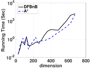
Finally we tested the scalability of our search algorithms on loopy graphical models. We generated synthetic models of different sizes. In particular, we generated regular k ⇥ k grid models, where k ranged from 5 to 26. We chose binary label (L = 2) and generated potentials randomly. Figure 5 shows the results when δ = 3 and M = 4. The performance of DFBnB and A* did not differ much in the comparison. When the model size was modest, they were both quite efficient. However, as the size further increased, their running times increased exponentially. Nevertheless, the results show that the search algorithms were scalable enough to handle models with almost 700 variables. In the future we plan to apply the methods to loopy models estimated from real world data.
6 Concluding Remarks
In this work, we developed two search algorithms to solve the M-Modes problem. M-Modes is a challenging problem due to its need to find solutions that not only have high probabilities but also need to be better than their local neighborhoods. The proposed search algorithms find global modes by directly searching the space of consistent local modes of all subgraphs. Such search is made possible using a new search operator designed to search a subgraph of variables at a time. The local modes of the subgraphs are generated and verified on the fly during the search. As a result, only a small number of local modes is explored by the search algorithms. Empirical evaluations against the state-of-the-art dynamic programming algorithm show that our search algorithms are much more efficient and scalable.
DFBnB and A* each has its own advantages and disadvantages. The depth-first search only needs to store search nodes on a single path at anytime. Given that only new boundary variables lead to new search nodes to be generated, the size of the stack can be bounded once the ordering of δ-subgraphs has been created. In practice, we found that the size of the stack is rather manageable. A*, however, has to store an open list of all frontier search nodes and may consume too much memory. On the other hand, due the best-first search nature, A* is guaranteed to expand fewer nodes than DFBnB; sometimes the difference can be huge. But due to the need to maintain a priority queue, each step of A* is more expensive than DFBnB. The practical performance of the two algorithms can thus only be determined empirically.
Our proposed search algorithms do not fully utilize the conditional independence structures of graphical models yet. As a future work, we plan to investigate how to formulate a search space that is more concise and efficient to search.
Acknowledgement
This research was supported by the NSF grants IIS-0953723, IIS-1219114, and a PSC-CUNY enhancement award.
@inproceedings{ijcai2016p505,
  title     = {Solving M-Modes Using Heuristic Search},
  author    = {Chen, Cong and Yuan, Changhe and Chen, Chao},
  booktitle = {Proceedings of the Twenty-Fifth International Joint Conference on
               Artificial Intelligence, {IJCAI-16}},
  publisher = {AAAI Press / International Joint Conferences on Artificial Intelligence},
  editor    = {Subbarao Kambhampati},
  pages     = {3584--3589},
  year      = {2016},
  month     = {7},
  url       = {https://ijcai.org/proceedings/2016/505},
}
TY - CPAPER TI - Solving M-Modes Using Heuristic Search AU - Chen, Cong AU - Yuan, Changhe AU - Chen, Chao T2 - Proceedings of the Twenty-Fifth International Joint Conference on Artificial Intelligence, IJCAI-16 PB - AAAI Press / International Joint Conferences on Artificial Intelligence PY - 2016 SP - 3584 EP - 3589 UR - https://ijcai.org/proceedings/2016/505 ER -Copied
Machine-readable versions of this paper, for tools and AI agents:





