
Swift: Compiled Inference for Probabilistic Programming Languages
Proceedings of the Twenty-Fifth International Joint Conference on Artificial Intelligence. Pages 3637-3644.
Abstract
A probabilistic program defines a probability measure over its semantic structures. One common goal of probabilistic programming languages (PPLs) is to compute posterior probabilities for arbitrary models and queries, given observed evidence, using a generic inference engine. Most PPL inference engines — even the compiled ones — incur significant runtime interpretation overhead, especially for contingent and open-universe models. This paper describes Swift, a compiler for the BLOG PPL. Swift-generated code incorporates optimizations that eliminate interpretation overhead, maintain dynamic dependencies efficiently, and handle memory management for possible worlds of varying sizes. Experiments comparing Swift with other PPL engines on avariety of inference problems demonstrate speedups ranging from 12x to326x.
- [Agrawal and Horgan, 1990] Hiralal Agrawal and Joseph R Hor- gan. Dynamic program slicing. In ACM SIGPLAN Notices, volume 25, pages 246-256. ACM, 1990.
- [Arora et al., 2010] Nimar S. Arora, Rodrigo de Salvo Braz, Erik B. Sudderth, and Stuart J. Russell. Gibbs sampling in open-universe stochastic languages. In UAI, pages 30-39. AUAI Press, 2010.
- [Chaganty et al., 2013] Arun Chaganty, Aditya Nori, and Sriram Rajamani. Efficiently sampling probabilistic programs via pro- gram analysis. In AISTATS, pages 153-160, 2013.
- [Cytron et al., 1989] Ron Cytron, Jeanne Ferrante, Barry K Rosen, Mark N Wegman, and F Kenneth Zadeck. An effi- cient method of computing static single assignment form. In Proceedings of the 16th ACM SIGPLAN-SIGACT symposium on Principles of programming languages, pages 25-35. ACM, 1989.
- [Goodman et al., 2008] Noah D. Goodman, Vikash K. Mans- inghka, Daniel M. Roy, Keith Bonawitz, and Joshua B. Tenen- baum. Church: A language for generative models. In UAI, pages 220-229, 2008.
- [Herbrich et al., 2007] Ralf Herbrich, Tom Minka, and Thore Graepel. Trueskill(tm): A bayesian skill rating system. In Advances in Neural Information Processing Systems 20, pages 569-576. MIT Press, January 2007.
- [Homan and Gelman, 2014] Matthew D Homan and Andrew Gelman. The no-u-turn sampler: Adaptively setting path lengths in hamiltonian monte carlo. The Journal of Machine Learning Research, 15(1):1593-1623, 2014.
- [Hur et al., 2014] Chung-Kil Hur, Aditya V. Nori, Sriram K. Ra- jamani, and Selva Samuel. Slicing probabilistic programs. In Proceedings of the 35th ACM SIGPLAN Conference on Pro- gramming Language Design and Implementation, PLDI '14, pages 133-144, New York, NY, USA, 2014. ACM.
- [Kazemi and Poole, 2016] Seyed Mehran Kazemi and David Poole. Knowledge compilation for lifted probabilistic infer- ence: Compiling to a low-level language. 2016.
- [Kucukelbir et al., 2015] Alp Kucukelbir, Rajesh Ranganath, An- drew Gelman, and David Blei. Automatic variational inference in Stan. In NIPS, pages 568-576, 2015.
- [LeCun et al., 1998] Yann LeCun, Léon Bottou, Yoshua Bengio, and Patrick Haffner. Gradient-based learning applied to doc- ument recognition. Proceedings of the IEEE, 86(11):2278- 2324, 1998.
- [Li et al., 2013] Lei Li, Bharath Ramsundar, and Stuart Russell. Dynamic scaled sampling for deterministic constraints. In AIS- TATS, pages 397-405, 2013.
- [Lunn et al., 2000] David J. Lunn, Andrew Thomas, Nicky Best, and David Spiegelhalter. WinBUGS -a Bayesian modelling framework: Concepts, structure, and extensibility. Statistics and Computing, 10(4):325-337, October 2000.
- [Mansinghka et al., 2013] Vikash K. Mansinghka, Tejas D. Kulkarni, Yura N. Perov, and Joshua B. Tenenbaum. Approx- imate Bayesian image interpretation using generative proba- bilistic graphics programs. In NIPS, pages 1520-1528, 2013.
- [McAllester et al., 2008] David McAllester, Brian Milch, and Noah D Goodman. Random-world semantics and syntactic in- dependence for expressive languages. Technical report, 2008.
- [Milch and Russell, 2006] Brian Milch and Stuart J. Russell. General-purpose MCMC inference over relational structures. In UAI. AUAI Press, 2006.
- [Milch et al., 2005a] Brian Milch, Bhaskara Marthi, Stuart Rus- sell, David Sontag, Daniel L. Ong, and Andrey Kolobov. BLOG: Probabilistic models with unknown objects. In IJCAI, pages 1352-1359, 2005. IJCAI
- [Milch et al., 2005b] Brian Milch, Bhaskara Marthi, David Son- tag, Stuart Russell, Daniel L. Ong, and Andrey Kolobov. Ap- proximate inference for infinite contingent Bayesian networks. In Tenth International Workshop on Artificial Intelligence and Statistics, Barbados, 2005.
- [Minka et al., 2014] T. Minka, J.M. Winn, J.P. Guiver, S. Web- ster, Y. Zaykov, B. Yangel, A. Spengler, and J. Bronskill. In- fer.NET 2.6, 2014.
- [Nori et al., 2014] Aditya V Nori, Chung-Kil Hur, Sriram K Ra- jamani, and Selva Samuel. R2: An efficient MCMC sampler for probabilistic programs. In AAAI Conference on Artificial Intelligence, 2014.
- [Pfeffer, 2001] Avi Pfeffer. IBAL: A probabilistic rational pro- gramming language. In In Proc. 17th IJCAI, pages 733-740. IJCAI
- [Pfeffer, 2009] Avi Pfeffer. Figaro: An object-oriented proba- bilistic programming language. Charles River Analytics Tech- nical Report, 2009.
- [Plummer, 2003] Martyn Plummer. JAGS: A program for anal- ysis of Bayesian graphical models using Gibbs sampling. In Proceedings of the 3rd International Workshop on Distributed Statistical Computing, volume 124, page 125. Vienna, 2003.
- [Ritchie et al., 2016] Daniel Ritchie, Andreas Stuhlmüller, and Noah D. Goodman. C3: Lightweight incrementalized MCMC for probabilistic programs using continuations and callsite caching. In AISTATS 2016, 2016.
- [Sanderson, 2010] Conrad Sanderson. Armadillo: An open source c++ linear algebra library for fast prototyping and com- putationally intensive experiments. 2010.
- [Shah et al., 2016] Rohin Shah, Emina Torlak, and Rastislav Bodik. SIMPL: A DSL for automatic specialization of infer- ence algorithms. arXiv preprint arXiv:1604.04729, 2016.
- [Stan Development Team, 2014] Stan Development Team. Stan Modeling Language Users Guide and Reference Manual, Ver- sion 2.5.0, 2014.
- [Tipping and Bishop, 1999] Michael E. Tipping and Chris M. Bishop. Probabilistic principal component analysis. Journal of the Royal Statistical Society, Series B, 61:611-622, 1999.
- [Tristan et al., 2014] Jean-Baptiste Tristan, Daniel Huang, Joseph Tassarotti, Adam C Pocock, Stephen Green, and Guy L Steele. Augur: Data-parallel probabilistic modeling. In NIPS, pages 2600-2608. 2014.
- [Wingate et al., 2011] David Wingate, Andreas Stuhlmueller, and Noah D Goodman. Lightweight implementations of proba- bilistic programming languages via transformational compila- tion. In International Conference on Artificial Intelligence and Statistics, pages 770-778, 2011.
- [Wood et al., 2014] Frank Wood, Jan Willem van de Meent, and Vikash Mansinghka. A new approach to probabilistic program- ming inference. In Proceedings of the 17th International con- ference on Artificial Intelligence and Statistics, pages 2-46, 2014.
- [Wu et al., 2014] Yi Wu, Lei Li, and Stuart J. Russell. BFiT: From possible-world semantics to random-evaluation seman- tics in open universe. In Neural Information Processing Sys- tems, Probabilistic Programming workshop, 2014.
- [Yang et al., 2014] Lingfeng Yang, Pat Hanrahan, and Noah D. Goodman. Generating efficient MCMC kernels from proba- bilistic programs. In AISTATS, pages 1068-1076, 2014.
References were extracted automatically from the PDF and may contain errors.
Full text extracted automatically from the PDF; figures, tables and equations may differ. The PDF is the version of record.
1 Introduction
Probabilistic programming languages (PPLs) aim to combine sufficient expressive power for writing real-world probability models with efficient, general-purpose inference algorithms that can answer arbitrary queries with respect to those models. One underlying motive is to relieve the user of the obligation to carry out machine learning research and implement new algorithms for each problem that comes along. Another is to support a wide range of cognitive functions in AI systems and to model those functions in humans.
General-purpose inference for PPLs is very challenging; they may include unbounded numbers of discrete and continuous variables, a rich library of distributions, and the ability to describe uncertainty over functions, relations, and the existence and identity of objects (so-called open-universe models). Existing PPL inference algorithms include likelihood weighting (LW) [Milch et al., 2005b], parental MetropolisHastings (PMH) [Milch and Russell, 2006; Goodman et al., 2008], generalized Gibbs sampling (Gibbs) [Arora et al., 2010], generalized sequential Monte Carlo [Wood et al., 2014], Hamiltonian Monte Carlo (HMC) [Stan Development Team, 2014], variational methods [Minka et al., 2014; Kucukelbir et al., 2015] and a form of approximate Bayesian computation [Mansinghka et al., 2013]. While better algorithms are certainly possible, our focus in this paper is on achieving orders-of-magnitude improvement in the execution efficiency of a given algorithmic process.
A PPL system takes a probabilistic program (PP) specifying a probabilistic model as its input and performs inference to compute the posterior distribution of a query given some observed evidence. The inference process does not (in general) execute the PP, but instead executes the steps of an inference algorithm (e.g., Gibbs) guided by the dependency structures implicit in the PP. In many PPL systems the PP exists as an internal data structure consulted by the inference algorithm at each step [Pfeffer, 2001; Lunn et al., 2000; Plummer, 2003; Milch et al., 2005a; Pfeffer, 2009]. This process is in essence an interpreter for the PP, similar to early Prolog systems that interpreted the logic program. Particularly when running sampling algorithms that involve millions of repetitive steps, the overhead can be enormous. A natural solution is to produce model-specific compiled inference code, but, as we show in Sec. 2, existing compilers for general open-universe models [Wingate et al., 2011; Yang et al., 2014; Hur et al., 2014; Chaganty et al., 2013; Nori et al., 2014] miss out on optimization opportunities and often produce inefficient inference code.
The paper analyzes the optimization opportunities for PPL compilers and describes the Swift compiler, which takes as input a BLOG program [Milch et al., 2005a] and one of three inference algorithms (LW, PMH, Gibbs) and generates target code for answering queries. Swift includes three main contributions: (1) elimination of interpretative overhead by joint analysis of the model structure and inference algorithm; (2) a dynamic slice maintenance method (FIDS) for incremental computation of the current dependency structure as sampling proceeds; and (3) efficient runtime memory management for maintaining the current-possible-world data structure as the number of objects changes. Comparisons between Swift and other PPLs on a variety of models demonstrate speedups ranging from 12x to 326x, leading in some cases to performance comparable to that of hand-built model-specific code. To the extent possible, we also analyze the contributions of each optimization technique to the overall speedup.
Although Swift is developed for the BLOG language, the overall design and the choices of optimizations can be applied to other PPLs and may bring useful insights to similar AI
systems for real-world applications.
2 Existing PPL Compilation Approaches
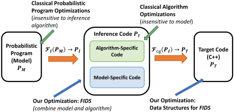
In a general purpose programming language (e.g., C++), the compiler compiles exactly what the user writes (the program). By contrast, a PPL compiler essentially compiles the inference algorithm, which is written by the PPL developer, as applied to a PP. This means that different implementations of the same inference algorithm for the same PP result in completely different target code.
As shown in Fig. 1, a PPL compiler first produces an intermediate representation combining the inference algorithm (I) and the input model (PM) as the inference code (PI ), and then compiles PI to the target code (PT ). Swift focuses on optimizing the inference code PI and the target code PT given a fixed input model PM.
Although there have been successful PPL compilers, these compilers are all designed for a restricted class of models with fixed dependency structures: see work by Tristan [2014] and the Stan Development Team [2014] for closed-world Bayes nets, Minka [2014] for factor graphs, and Kazemi and Poole [2016] for Markov logic networks.
Church [Goodman et al., 2008] and its variants [Wingate et al., 2011; Yang et al., 2014; Ritchie et al., 2016] provide a lightweight compilation framework for performing the Metropolis-Hastings algorithm (MH) over general openuniverse probability models (OUPMs). However, these approaches (1) are based on an inefficient implementation of MH, which results in overhead in PI, and (2) rely on inefficient data structures in the target code PT .
For the first point, consider an MH iteration where we are proposing a new possible world w0 from w accoding to the proposal g(·) by resampling random variable X from v to v0 . The computation of acceptance ratio ↵ follows
Since only X is resampled, it is sufficient to compute ↵ using merely the Markov blanket of X, which leads to a much simplified formula for ↵ from Eq.(1) by cancelling terms in Pr[w] and Pr[w0 ]. However, when applying MH for a contingent model, the Markov blanket of a random variable cannot be determined at compile time since the model dependencies vary during inference. This introduces tremendous runtime overhead for interpretive systems (e.g., BLOG, Figaro),
1 type Ball; type Draw; type Color; //3 types 2 distinct Color Blue, Green; //two colors 3 distinct Draw D[2]; //two draws: D[0], D[1] 4 #Ball ~ UniformInt(1,20);//unknown # of balls 5 random Color color(Ball b) //color of a ball 6 ~ Categorical({Blue -> 0.9, Green -> 0.1}); 7 random Ball drawn(Draw d) 8 ~ UniformChoice({b for Ball b}); 9 obs color(drawn(D[0])) = Green; // drawn ball is green 10 query color(drawn(D[1])); // query1 type Cluster; type Data; 2 distinct Data D[20]; // 20 data points 3 #Cluster ~ Poisson(4); // number of clusters 4 random Real mu(Cluster c) ~ Gaussian(0,10); //cluster mean 5 random Cluster z(Data d) 6 ~ UniformChoice({c for Cluster c}); 7 random Real x(Data d) ~ Gaussian(mu(z(d)), 1.0); // data which track all the dependencies at runtime even though typically only a tiny portion of the dependency structure may change per iteration. Church simply avoids keeping track of dependencies and uses Eq.(1), including a potentially huge overhead for redundant probability computations.
8 obs x(D[0]) = 0.1; // omit other data points 9 query size({c for Cluster c}); Figure 3: The infinite Gaussian mixture model For the second point, in order to track the existence of the variables in an open-universe model, similar to BLOG, Church also maintains a complicated dynamic string-based hashing scheme in the target code, which again causes interpretation overhead.
generic approach is Monte-Carlo sampling, such as likelihood weighting [Milch et al., 2005a] (LW) and MetropolisHastings algorithm (MH). For LW, the main idea is to sample every random variable from its prior per iteration and colLastly, techniques proposed by Hur et al. [2014], Chaganty et al. [2013] and Nori et al. [2014] primarily focus on optimizing PM by analyzing the static properties of the input PP, which are complementary to Swift.
lect weighted samples for the queries, where the weight is the
likelihood of the evidences. For MH, the high-level procedure 3 Background
of the algorithm is summarized in Alg. 1. M denotes an input BLOG program (or model), E its evidence, Q a query, N denotes the number of samples, W denotes a possible world, W(x) is the value of x in possible world W , Pr[x♣W ] denotes the conditional probability of x in W, and Pr[W] denotes the likelihood of possible world W. In particular, when the proThis paper focuses on the BLOG language, although our approach also applies to other PPLs with equivalent semantics [McAllester et al., 2008; Wu et al., 2014]. Other PPLs can be also converted to BLOG via static single assignment form (SSA form) transformation [Cytron et al., 1989; Hur et al., 2014].
algorithm becomes the parental MH algorithm (PMH). Our 3.1 The BLOGLanguage
posal distribution g in Alg.1 is the prior of every variable, the
discussion in the paper focuses on LW and PMH but our proposed solution applies to other Monte-Carlo methods as well. 4 The Swift Compiler Swift has the following design goals for handling openuniverse probabilistic models. ÷ Provide a general framework to automatically and efficiently (1) track the exact Markov blanket for each random variable and (2) maintain the minimum set of The BLOG language [Milch et al., 2005a] defines probability measures over first-order (relational) possible worlds; in this sense it is a probabilistic analogue of first-order logic. A BLOG program declares types for objects and defines distributions over their numbers, as well as defining distributions for the values of random functions applied to objects. Observation statements supply evidence, and a query statement specifies the posterior probability of interest. A random variable in BLOG corresponds to the application of a random function to specific objects in a possible world. BLOG naturally supports open universe probability models (OUPMs) and context-specific dependencies.
Algorithm 1: Metropolis-Hastings algorithm (MH) Input: M, E, Q, N; Output: samples H 1 initialize a possible world W0 with E satisfied; 2 for i 1 to N do 3 randomly pick a variable x fromWi-1 ; 4 Wi Wi-1 and v Wi-1(x); 5 propose a value v0 for x via proposal g; 6 Wi(x) v0 and ensure Wi is supported; 7 ↵ min ⇣1↪ g(v0!v)Pr[Wi] g(v!v0) Pr[Wi-1] ⌘ ; Fig. 2 demonstrates the open-universe urn-ball model. In this version the query asks for the color of the next random pick from an urn given the colors of balls drawn previously. Line 4 is a number statement stating that the number variable #Ball, corresponding to the total number of balls, is uniformly distributed between 1 and 20. Lines 5-6 declare a random function color(·), applied to balls, picking Blue or Green with a biased probability. Lines 7-8 state that each draw chooses a ball at random from the urn, with replacement.
8 if rand(0↪ 1) ≥ ↵ then Wi Wi-1 H H + (Wi(Q)); Fig. 3 describes another OUPM, the infinite Gaussian mixture model (1-GMM). The model includes an unknown
÷
Fo
(Fra
gene
goal,
code
Fo
dem
discu
Sec.
Swift
only
conti
4.1
Our
thou
inclu
adapt
ing (
and
Dyn
Dyna
a dy
varia
com
piler)
and
durin
Fo
input
is us
and (
the c
infer
D
is to
struc
targe
Fo
x(d)
doub
//
me
//
va
re
Sinc
mu(
Nota
denc
non-
9 obs color(drawn(D[0])) = Green; // drawn ball is green
10 query color(drawn(D[1])); // query
Figure 2: The urn-ball model
1 type Cluster; type Data; 2 distinct Data D[20]; // 20 data points 3 #Cluster ~ Poisson(4); // number of clusters 4 random Real mu(Cluster c) ~ Gaussian(0,10); //cluster mean 5 random Cluster z(Data d) 6 ~ UniformChoice({c for Cluster c}); 7 random Real x(Data d) ~ Gaussian(mu(z(d)), 1.0); // data 8 obs x(D[0]) = 0.1; // omit other data points 9 query size({c for Cluster c}); Figure 2: The urn-ball modelgeneric approach is Monte-Carlo sampling, such as likeliAlgorithm 1: Metropolis-Hastings algorithm (MH)
hood weighting [Milch et al., 2005a] (LW) and MetropolisHastings algorithm (MH). For LW, the main idea is to sample every random variable from its prior per iteration and collect weighted samples for the queries, where the weight is the likelihood of the evidences. For MH, the high-level procedure of the algorithm is summarized in Alg. 1. M denotes an input BLOG program (or model), E its evidence, Q a query, N denotes the number of samples, W denotes a possible world, W(x) is the value of x in possible world W , Pr[x♣W ] denotes the conditional probability of x in W, and Pr[W] denotes the likelihood of possible world W. In particular, when the proposal distribution g in Alg.1 is the prior of every variable, the Input: M, E, Q, N; Output: samples H 1 initialize a possible world w(0) with E satisfied; 2 for i 1 to N do 3 randomly pick a variable X from w(i-1) ; 4 w(i) w(i-1) and v X(w(i-1) ); 5 propose a value v0 for X via proposal g; 6 X(w(i) ) v0 and ensure w(i) is self-supporting; 7 ↵ min ⇣1↪ g(v0!v)Pr[w(i) ] g(v!v0) Pr[w(i-1) ] ⌘ ; 8 if rand(0↪ 1) ≥ ↵ then w(i) w(i-1) ; 9 H H + (Q(w(i) )); Figure 3: The infinite Gaussian mixture model generic approach is Monte-Carlo sampling, such as likelihood weighting [Milch et al., 2005a] (LW) and MetropolisHastings algorithm (MH). For LW, the main idea is to sample every random variable from its prior per iteration and collect weighted samples for the queries, where the weight is the likelihood of the evidences. For MH, the high-level procedurealgorithm becomes the parental MH algorithm (PMH). Our
of the algorithm is summarized in Alg. 1. M denotes an in-
discussion in the paper focuses on LW and PMH but our pro-
put BLOG program (or model), E its evidence, Q a query, N
posed solution applies to other Monte-Carlo methods as well. number of clusters as stated in line 3, which is to be inferred from the data. denotes the number of samples, W denotes a possible world, W(x) is the value of x in possible world W , Pr[x♣W ] denotes
the conditional probability of x in W, and Pr[W] denotes the
Swift has the following design goals for handling open3.2 Generic Inference Algorithms likelihood of possible world W. In particular, when the pro-
4 The Swift Compiler
universe probabilistic models. ÷ Provide a general framework to automatically and efficiently (1) track the exact Markov blanket for each random variable and (2) maintain the minimum set of Algorithm 1: Metropolis-Hastings algorithm (MH) Input: M, E, Q, N; Output: samples H 1 initialize a possible world W0 with E satisfied; 2 for i 1 to N do 3 randomly pick a variable x fromWi-1 ; 4 Wi Wi-1 and v Wi-1(x); 5 propose a value v0 for x via proposal g; 6 Wi(x) v0 and ensure Wi is supported; 7 ↵ min ⇣1↪ g(v0!v)Pr[Wi] g(v!v0) Pr[Wi-1] ⌘ ; 8 if rand(0↪ 1) ≥ ↵ then Wi Wi-1 H H + (Wi(Q)); All PPLs need to infer the posterior distribution of a query given the observed evidence. The great majority of PPLs use Monte Carlo sampling methods such as likelihood weighting (LW) and Metropolis-Hastings MCMC (MH). LW samples unobserved random variables sequentially in topological order, conditioned on evidence and sampled values earlier in the sequence; each complete sample is weighted by the likelihood of the evidence variables appearing in the sequence. The MH algorithm is summarized in Alg. 1. M denotes a BLOG model, E its evidence, Q a query, N the number of samples, w a possible world, X(w) the value of random variable X in w, Pr[X(w)♣w-X] denotes the conditional probability of X in w, and Pr[w] denotes the likelihood of possible world w. In particular, when the proposal distribution g in Alg.1 samples a variable conditioned on its parents, the algorithm becomes the parental MH algorithm (PMH). Our discussion in the paper focuses on LW and PMH but our proposed solution applies to other Monte Carlo methods as well. posal distribution g in Alg.1 is the prior of every variable, the algorithm becomes the parental MH algorithm (PMH). Our discussion in the paper focuses on LW and PMH but our proposed solution applies to other Monte-Carlo methods as well. 4 The Swift Compiler Swift has the following design goals for handling openuniverse probabilistic models. ÷ Provide a general framework to automatically and efficiently (1) track the exact Markov blanket for each random variable and (2) maintain the minimum set of random variables necessary to evaluate the query and Algorithm 1: Metropolis-Hastings algorithm (MH) Input: M, E, Q, N; Output: samples H 1 initialize a possible world W0 with E satisfied; 2 for i 1 to N do
3
4 The Swift Compiler 4 Wi Wi-1 and v Wi-1(x); 5 propose a value v0 for x via proposal g;
randomly pick a variable x fromWi-1 ;
Swift has the following design goals for handling openuniverse probability models. 6 Wi(x) v0 and ensure Wi is supported; 7 ↵ min ⇣1↪ g(v0!v)Pr[Wi] g(v!v0) Pr[Wi-1] ⌘ ;
- ÷ Provide a general framework to automatically and efficiently (1) track the exact Markov blanket for each random variable and (2) maintain the minimum set of random variables necessary to evaluate the query and the evidence (the dynamic slice [Agrawal and Horgan, 1990], or equivalently the minimum self-supporting partial world [Milch et al., 2005a]). if rand(0↪ 1) ≥ ↵ then Wi Wi-1 H H + (Wi(Q));
8
structures for Monte Carlo sampling algorithms to avoid
interpretive overhead at runtime.
the evidence (the dynamic slice [Agrawal and Horgan,
1990], or equivalently the minimum self-supported par-
tial world [Milch et al., 2005a]).
For the first goal, we propose a novel framework FIDS
(Framework of Incrementally updating Dynamic Slices) for
generating the inference code (PI in Fig. 1). For the second
- goal, we carefully choose data structures in the target C++ code (PT ). For convenience, r.v. is short for random variable. We ÷ Provide efficient memory management and fast data structures for Monte Carlo sampling algorithms to avoid interpretive overhead at runtime. ÷ Provide efficient memory management and fast data structures for Monte Carlo sampling algorithms to avoid interpretive overhead at runtime.
demonstrate examples of compiled code in the following discussion: the inference code (PI) generated by FIDS in Sec. 4.1 are all in pseudo-code while the target code (PT ) by Swift shown in Sec. 4.2 are in C++. Due to limited space, we only show the detailed transformation rules for the adaptive contingency updating (ACU) technique and omit the others. For the first goal, we propose a novel framework, FIDS (Framework for Incrementally updating Dynamic Slices), for generating the inference code (PI in Fig. 1). For the second goal, we carefully choose data structures in the target C++ code (PT ). For the first goal, we propose a novel framework FIDS (Framework of Incrementally updating Dynamic Slices) for generating the inference code (PI in Fig. 1). For the second goal, we carefully choose data structures in the target C++ code (PT ).
4.1 Optimizations in FIDS Our discussion in this section focuses on LW and PMH, although FIDS can be also applied to other algorithms. FIDS includes three optimizations: dynamic backchaining (DB), adaptive contingency updating (ACU) and reference counting (RC). DB is applied to both LW and PMH while ACU For convenience, r.v. is short for random variable. We demonstrate examples of compiled code in the following discussion: the inference code (PI) generated by FIDS in Sec. 4.1 is in pseudo-code while the target code (PT ) by Swift shown in Sec. 4.2 is in C++. Due to limited space, we show the detailed transformation rules only for the adaptive contingency updating (ACU) technique and omit the others. For convenience, r.v. is short for random variable. We demonstrate examples of compiled code in the following discussion: the inference code (PI) generated by FIDS in Sec. 4.1 are all in pseudo-code while the target code (PT ) by Swift shown in Sec. 4.2 are in C++. Due to limited space, we only show the detailed transformation rules for the adaptive contingency updating (ACU) technique and omit the others.
and RC are particularly for PMH.
Dynamic backchaining Dynamic backchaining (DB) aims to incrementally construct a dynamic slice in each LW iteration and only sample those variables necessary at runtime. DB is adaptive from idea of compiling lazy evaluation (also similar to the Prolog compiler): in each iteration, DB backtracks from the evidence and query and samples a r.v. only when its value is required Our discussion in this section focuses on LW and PMH, although FIDS can be also applied to other algorithms. FIDS includes three optimizations: dynamic backchaining (DB), adaptive contingency updating (ACU), and reference counting (RC). DB is applied to both LW and PMH while ACU and RC are specific to PMH. Our discussion in this section focuses on LW and PMH, although FIDS can be also applied to other algorithms. FIDS includes three optimizations: dynamic backchaining (DB), adaptive contingency updating (ACU) and reference counting (RC). DB is applied to both LW and PMH while ACU and RC are particularly for PMH.
4.1 Optimizations in FIDS 4.1 Optimizations in FIDS
during inference. Dynamic backchaining Dynamic backchaining
For every r.v. declaration random T X ⇠ CX; in the input PP, FIDS generates a getter function get X(), which is used to (1) sample a value for X from its declaration CX and (2) memoize the sampled value for later references in the current iteration. Whenever a r.v. is referred to during inference, its getter function will be evoked. DB is the fundamental technique for Swift. The key insight Dynamic backchaining (DB) [Milch et al., 2005a] constructs a dynamic slice incrementally in each LW iteration and samples only those variables necessary at runtime. DB in Swift is an example of compiling lazy evaluation: in each iteration, DB backtracks from the evidence and query and samples an r.v. only when its value is required during inference. Dynamic backchaining (DB) aims to incrementally construct a dynamic slice in each LW iteration and only sample those variables necessary at runtime. DB is adaptive from idea of compiling lazy evaluation (also similar to the Prolog compiler): in each iteration, DB backtracks from the evidence and query and samples a r.v. only when its value is required
is to replace the dependency look-up in some interpretive data structure by direct machine address/instruction seeking in the target executable file. For example, the inference code for the getter function of x(d) in the1-GMMmodel (Fig. 3) is shown below. double get_x(Data d) { For every r.v. declaration random T X ⇠ CX; in the input PP, FIDS generates a getter function get X(), which is used to (1) sample a value for X from its declaration CX and (2) memoize the sampled value for later references in the current iteration. Whenever an r.v. is referred to during inference, its getter function will be evoked. during inference. For every r.v. declaration random T X ⇠ CX; in the input PP, FIDS generates a getter function get X(), which is used to (1) sample a value for X from its declaration CX and (2) memoize the sampled value for later references in the current iteration. Whenever a r.v. is referred to during
// some code memoizing the sampled value memoization; // if not sampled, sample a new value val = sample_gaussian(get_mu(get_z(d)),1); return val; } Compiling DB is the fundamental technique for Swift. The key insight is to replace dependency look-ups and method invocations from some internal PP data structure with direct machine address accessing and branching in the target executable file. inference, its getter function will be evoked. DB is the fundamental technique for Swift. The key insight is to replace the dependency look-up in some interpretive data structure by direct machine address/instruction seeking in the target executable file.
dency look-up is ever required at runtime to discover those non-empty clusters. double get_x(Data d) { // some code memoizing the sampled value memoization; // if not sampled, sample a new value val = sample_gaussian(get_mu(get_z(d)),1); return val; }Since get_z( · ) is called before get_mu( · ), only those mu(c) corresponding to non-empty clusters will be sampled. Notably, with the inference code above, no explicit depenFor example, the inference code for the getter function of x(d) in the1-GMMmodel (Fig. 3) is shown below. For example, the inference code for the getter function of x(d) in the1-GMMmodel (Fig. 3) is shown below.
Since get_z( · ) is called before get_mu( · ), only those mu(c) corresponding to non-empty clusters will be sampled. Notably, with the inference code above, no explicit dependency look-up is ever required at runtime to discover those non-empty clusters. memoization denotes some pseudo-code snippet for performing memoization. Since get_z(·) is called before get_mu(·), only those mu(c) corresponding to non-empty clusters will be sampled. Notably, with the inference code above, no explicit dependency look-up is ever required at runtime to discover those non-empty clusters.
When sampling a number variable, we need to allocate memory for the associated variables. For example, in the urnball model (Fig. 2), we need to allocate memory for color(b)
When sampling a number variable, we need to allocate
memory for the associated variables, i.e., in the urn-ball
When sampling a number variable, we need to allocate
memory for the associated variables, i.e., in the urn-ball
model (Fig. 2), we need to allocate memory for color(b) af-
model (Fig. 2), we need to allocate memory for color(b) af-
ter sampling #Ball. The corresponding generated code is
int get_num_Ball() {
after sampling #Ball. The corresponding generated inference code is shown below. ter sampling #Ball. The corresponding generated code is shown below. shown below.
int get_num_Ball() { // some code for memoization memoization; // sample a value val = sample_uniformInt(1,20); // some code allocating memory for color allocate_memory_color(val); return val; } // some code for memoization memoization; // sample a value val = sample_uniformInt(1,20); // some code allocating memory for color allocate_memory_color(val); return val; }allocate_memory_color(val) denotes some pseudocode segment for allocating val chunks of memory for the values of color(b). allocate_memory_color(val) denotes some pseudocode segment for allocating val chunks of memory for the values of color(b). allocate_memory_color(val) denotes some pseudocode segment for allocating val chunks of memory for the values of color(b).
Reference Counting Reference Counting Reference Counting
For a r.v. being tracked, say X, RC maintains a reference counter cnt(X) defined by cnt(X) = ♣Ch(X♣W)♣. Ch(X♣W) denote the children of X in the possible world W. When cnt(X) becomes zero, X is removed from W; when cnt(X) become positive, X is instantiated and added back to W. This procedure is performed recursively. For an r.v. being tracked, say X, RC maintains a reference counter cnt(X) defined by cnt(X) = ♣Chw(X)♣. Chw(X) denote the children of X in the possible world w. When cnt(X) becomes zero, X is removed from w; when cnt(X) become positive, X is instantiated and added back to w. This procedure is performed recursively. For a r.v. being tracked, say X, RC maintains a reference counter cnt(X) defined by cnt(X) = ♣Ch(X♣W)♣. Ch(X♣W) denote the children of X in the possible world W. When cnt(X) becomes zero, X is removed from W; when cnt(X) become positive, X is instantiated and added back to W. This procedure is performed recursively.
Reference counting (RC) generalize the idea of DB to incrementally maintain the dynamic slice in PMH. RC is a efficient compilation strategy for the interpretive BLOG to dynamically maintain references to variables and exclude those without any references from the current possible world with minimal runtime overhead. RC is also similar to dynamic garbage collection in programming language community. Reference counting (RC) generalize the idea of DB to incrementally maintain the dynamic slice in PMH. RC is an efficient compilation strategy for the interpretive BLOG to dynamically maintain references to variables and exclude those without any references from the current possible world with minimal runtime overhead. RC is also similar to dynamic garbage collection in programming language community. Reference counting (RC) generalize the idea of DB to incrementally maintain the dynamic slice in PMH. RC is a efficient compilation strategy for the interpretive BLOG to dynamically maintain references to variables and exclude those without any references from the current possible world with minimal runtime overhead. RC is also similar to dynamic garbage collection in programming language community.
Tracking references to every r.v. might cause unnecessary overhead. For example, for classical Bayes nets, RC never excludes any variables. Hence, as a trade-off, Swift only counts references in open-universe models, particularly, to those variables associated with number variables (i.e., color(b) in the urn-ball model). Tracking references to every r.v. might cause unnecessary overhead. For example, for classical Bayes nets, RC never excludes any variables. Hence, as a trade-off, Swift only counts references in open-universe models, particularly, to those variables associated with number variables (e.g., color(b) in the urn-ball model). Tracking references to every r.v. might cause unnecessary overhead. For example, for classical Bayes nets, RC never excludes any variables. Hence, as a trade-off, Swift only counts references in open-universe models, particularly, to those variables associated with number variables (i.e., color(b) in the urn-ball model).
Take the urn-ball model as an example. When resampling drawn(d) and accepting the proposed value v, the generated code for accepting the proposal will be Take the urn-ball model as an example. When resampling drawn(d) and accepting the proposed value v, the generated code for accepting the proposal will be Take the urn-ball model as an example. When resampling drawn(d) and accepting the proposed value v, the generated code for accepting the proposal will be
void inc_cnt(X) { if (cnt(X) == 0) W.add(X); cnt(X) = cnt(X) + 1; } void dec_cnt(X) { cnt(X) = cnt(X) - 1; if (cnt(X) == 0) W.remove(X); } void accept_value_drawn(Draw d, Ball v) { // code for updating dependencies omitted dec_cnt(color(val_drawn(d))); val_drawn(d) = v; void inc_cnt(X) { if (cnt(X) == 0) W.add(X); cnt(X) = cnt(X) + 1; } void dec_cnt(X) { cnt(X) = cnt(X) - 1; if (cnt(X) == 0) W.remove(X); } void accept_value_drawn(Draw d, Ball v) { // code for updating dependencies omitted dec_cnt(color(val_drawn(d))); val_drawn(d) = v; inc_cnt(color(v)); }inc_cnt(color(v)); }
The function inc_cnt(X) and dec_cnt(X) update the references to X. The function accept_value_drawn() is specialized to r.v. drawn(d): Swift analyzes the input proThe function inc_cnt(X) and dec_cnt(X) update the references to X. The function accept_value_drawn() is specialized to r.v. drawn(d): Swift analyzes the input program and generates specialized codes for different variables. The function inc_cnt(X) and dec_cnt(X) update the references to X. The function accept_value_drawn() is specialized to r.v. drawn(d): Swift analyzes the input program and generates specialized codes for different variables.
gram and generates specialized codes for different variables.
Adaptive contingency updating Adaptive contingency updating
Adaptive contingency updating The goal of ACU is to incrementally maintain the Markov The goal of ACU is to incrementally maintain the Markov Blanket for every r.v. with minimal efforts. The goal of ACU is to incrementally maintain the Markov Blanket for every r.v. with minimal efforts.
Blanket for every r.v. with minimal efforts. CX denotes the declaration of r.v. X in the input PP; Parw(X) denote the parents of X in the possible world w; w[X v] denotes the new possible world derived from w by only changing the value of X to v. Note that deriving CX denotes the declaration of r.v. X in the input PP;
Par(X♣W) denote the parents of X in the possible world
CX denotes the declaration of r.v. X in the input PP;
W; W(X v) denotes the new possible world derived from
W by only changing the value of X to v. Note that deriving
Par(X♣W) denote the parents of X in the possible world
W; W(X v) denotes the new possible world derived from
W by only changing the value of X to v. Note that deriving W(X v) may require instantiating new variables not exW(X v) may require instantiating new variables not existing in W due to dependency changes. w[X v] may require instantiating new variables not existing in w due to dependency changes.
ground truth Ch(X♣W) under the current PWW. With a proposed possible world (PW) W(X v), it is easy to add all missing dependencies from a particular variable U. That is, for a r.v. U and every r.v. V 2 Par(U♣W), we can verify whether U 2 Ch(V ♣W) and add U to Ch(X) if U 62 Ch(X). Therefore, the key step becomes tracking the set of variables, ∆(W(X v)), which will have a different With a proposed possible world (PW) W(X v), it is easy to add all missing dependencies from a particular variable U. That is, for a r.v. U and every r.v. V 2 Par(U♣W), we can verify whether U 2 Ch(V ♣W) and add U to Ch(X) if U 62 Ch(X). Therefore, the key step becomes tracking the set of variables, ∆(W(X v)), which will have a different set of parents inW(X v). With a proposed possible world (PW) w0 = w[X v], it is easy to add all missing dependencies from a particular r.v. U. That is, for an r.v. U and every r.v. V 2 Parw0(U), since U must be in Chw0 (V ), we can keep Ch(V) up-to-date by adding U to Ch(V) if U 62 Ch(V). Therefore, the key step is tracking the set of variables, ∆(w[X v]), which will have a set of parents in w[X v] different fromw.
isting in W due to dependency changes. Computing Par(X♣W) for X is straightforward by executing its generation process, CX, within W, which is often inexpensive. Hence, the principal challenge for maintaining the Markov blanket is to efficiently maintain a children set Ch(X) for each r.v. X with the aim of keeping identical the Computing Par(X♣W) for X is straightforward by executing its generation process, CX, within W, which is often inexpensive. Hence, the principal challenge for maintaining the Markov blanket is to efficiently maintain a children set Ch(X) for each r.v. X with the aim of keeping identical the ground truth Ch(X♣W) under the current PWW. Computing Parw(X) for X is straightforward by executing its generation process, CX, within w, which is often inexpensive. Hence, the principal challenge for maintaining the Markov blanket is to efficiently maintain a children set Ch(X) for each r.v. X with the aim of keeping identical to the true set Chw(X) for the current possible world w.
any value v. We call this over-approximation the contingent set Cont(X♣W). Note that for every r.v. V with dependency that changes in W(X v), X must be reached in the condition of a control statement on the execution path of CV within W, namely ∆(W(X v)) ✓ Ch(X♣W). One straightforward idea is any value v. We call this over-approximation the contingent set Cont(X♣W). Note that for every r.v. V with dependency that changes in W(X v), X must be reached in the condition of a control statement on the execution path of CV within W, namely ∆(W(X v)) ✓ Ch(X♣W). One straightforward idea is set Cont(X♣W) = Ch(X♣W). However, this leads to too Note that for every r.v. U with dependency that changes in w(X v), X must be reached in the condition of a control statement on the execution path of CU within w. This implies ∆(w[X v]) ✓ Chw(X). One straightforward idea is set Contw(X) = Chw(X). However, this leads to too much overhead. For example, ∆(·) should be always empty for models with fixed dependencies.
∆(W(X v)) = ¶Y : Par(Y ♣W) 6= Par(Y ♣W(X v))♦ Precisely computing ∆(W(X v)) is very expensive at runtime but computing an upper bound for ∆(W(X v)) does not influence the correctness of the inference code. Therefore, we proceed to find an upper bound that holds for ¶Y : Par(Y ♣W) 6= Par(Y ♣W(X v))♦ Precisely computing ∆(W(X v)) is very expensive at runtime but computing an upper bound for ∆(W(X v)) does not influence the correctness of the inference code. Therefore, we proceed to find an upper bound that holds for Precisely computing ∆(w[X v]) is very expensive at runtime but computing an upper bound for ∆(w[X v]) does not influence the correctness of the inference code. Therefore, we proceed to find an upper bound that holds for any value v. We call this over-approximation the contingent set Contw(X).
set Cont(X♣W) = Ch(X♣W). However, this leads to too much overhead. For example, ∆( · ) should be always empty for models with fixed dependency. much overhead. For example, ∆( · ) should be always empty for models with fixed dependency. Another approach is to first find out the set of switching Another approach is to first find out the set of switching variables SX for every r.v. X, which is defined by
SX = ¶Y : 9W↪ v Par(X♣W) 6= Par(X♣W(Y v))♦↪ SX = ¶Y : 9W↪ v Par(X♣W) 6= Par(X♣W(Y v))♦↪ This brings an immediate advantage: SX can be statically This brings an immediate advantage: SX can be statically computed at compile time. However, computing SX is NPComplete 1 .
This brings an immediate advantage: SX can be statically computed at compile time. However, computing SX is NPComplete 1 . SX by taking computed at compile time. However, computing SX is NPComplete 1 . Our solution is to derive the approximation b SX by taking Our solution is to derive the approximation b SX by taking the union of free variables of if/case conditions, function arguments, and set expression conditions in CX, and then set
set Cont(X) for every r.v. X corresponding to true contingent set Cont(X♣W) under the current PW W. Cont(X) can be incrementally updated. Back to the original focus of ACU, suppose we are adding new the dependencies in the new PWW(X x). There are three steps to accomplish the goal: (1) enumerating all the gent set Cont(X♣W) under the current PW W. Cont(X) can be incrementally updated. Back to the original focus of ACU, suppose we are adding new the dependencies in the new PWW(X x). There are three steps to accomplish the goal: (1) enumerating all the 1 Since the declaration CX may contain arbitrary boolean formuBack to the original focus of ACU, suppose we are adding new the dependencies in the newPWw0 = w[X v]. There are three steps to accomplish the goal: (1) enumerating all the variables U 2 Cont(X), (2) for all V 2 Parw0(U), add U to Ch(V), and (3) for all V 2 Parw0(U) \ b SU, add U to Cont(V). These steps can be also repeated in a similar way to remove the vanished dependencies.
guments, and set expression conditions in CX, and then set Cont(X♣W) = ¶Y : Y 2 Ch(X♣W) ^X 2 b SY ♦▷ Cont(X♣W) is a function of the sampling variable X and the current PWW. Likewise, we maintain a runtime contingent Cont(X♣W) = ¶Y : Y 2 Ch(X♣W) ^X 2 b SY ♦▷ Cont(X♣W) is a function of the sampling variable X and the current PWW. Likewise, we maintain a runtime contingent set Cont(X) for every r.v. X corresponding to true continContw(X) = ¶Y : Y 2 Chw(X) ^X 2 b Contw(X) is a function of the sampling variable X and the current PW w. Likewise, for every r.v. X, we maintain a runtime contingent set Cont(X) identical to the true set Contw(X) under the current PW w. Cont(X) can be incrementally updated as well.
1 Since the declaration CX may contain arbitrary boolean formulas, one can reduce the 3-SAT problem to computing SX. las, one can reduce the 3-SAT problem to computing SX. Take the 1-GMMmodel (Fig. 3) as an example , when resampling z(d), we need to change the dependency of r.v. x(d)
1 Since the declaration CX may contain arbitrary boolean formulas, one can reduce the 3-SAT problem to computing SX.
{ Fcc(C↪ Id↪ ¶♦) }
void Id::accept_value(T v)
{ for(u in Cont(Id)) u.del_from_Ch();
Id = v;
Fc(M = random T Id([T Id ,]⇤ ) ⇠ C) =
for(u in Cont(Id)) u.add_to_Ch(); }
void Id::add_to_Ch()
Fc(M = random T Id([T Id ,]⇤ ) ⇠ C) = void Id::add_to_Ch() { Fcc(C↪ Id↪ ¶♦) } void Id::accept_value(T v) { for(u in Cont(Id)) u.del_from_Ch(); Id = v; for(u in Cont(Id)) u.add_to_Ch(); } Fcc(C = Exp↪ X↪ seen) = Fcc(Exp↪ X↪ seen) Fcc(C = Dist(Exp)↪ X↪ seen) = Fcc(Exp↪ X↪ seen) Fcc(C = if (Exp) then C1 else C2↪ X↪ seen) = Fcc(Exp↪ X↪ seen); if (Exp) { Fcc(C1↪X↪ seen [FV (Exp)); } else { Fcc(C2↪X↪ seen [FV (Exp)); } Fcc(Exp↪ X↪ seen) = /* emit a line of code for every r.v. U in the corresponding set */ 8 U 2 ((FV (Exp) \ b SX)∩seen) : Cont(U) += X; 8 U 2 (FV (Exp)∩seen) : Ch(U) += X; Fcc(C = Exp↪ X↪ seen) = Fcc(Exp↪ X↪ seen) Fcc(C = Dist(Exp)↪ X↪ seen) = Fcc(Exp↪ X↪ seen) Fcc(C = if (Exp) then C1 else C2↪ X↪ seen) = Fcc(Exp↪ X↪ seen) if (Exp) { Fcc(C1↪X↪ seen [FV (Exp)) } else { Fcc(C2↪X↪ seen [FV (Exp)) } Fcc(Exp↪ X↪ seen) = /* emit a line of code for every r.v. U in the corresponding set */ 8 U 2 ((FV (Exp) \ b SX)∩seen) : Cont(U) += X; 8 U 2 (FV (Exp)∩seen) : Ch(U) += X; Figure 4: Transformation rules for outputting inference code with ACU. FV (Expr) denotes the free variables in Expr. We assume the switching variables b SX have already been computed. The rules for number statements and case statements are not shown for conciseness-they are analogous to the rules for random variables and if statements respectively. { Fcc(C↪ Id↪ ¶♦) } void Id::accept_value(T v) { for(u in Cont(Id)) u.del_from_Ch(); Id = v; for(u in Cont(Id)) u.add_to_Ch(); } Fcc(C = Exp↪ X↪ seen) = Fcc(Exp↪ X↪ seen) Fcc(C = Dist(Exp)↪ X↪ seen) = Fcc(Exp↪ X↪ seen) Fcc(C = if (Exp) then C1 else C2↪ X↪ seen) = Fcc(Exp↪ X↪ seen) if (Exp) { Fcc(C1↪X↪ seen [FV (Exp)) } else { Fcc(C2↪X↪ seen [FV (Exp)) } Fcc(Exp↪ X↪ seen) = /* emit a line of code for every r.v. U in the corresponding set */ 8 U 2 ((FV (Exp) \ b SX)∩seen) : Cont(U) += X; 8 U 2 (FV (Exp)∩seen) : Ch(U) += X; Figure 4: Transformation rules for outputting inference code with ACU. FV (Expr) denotes the free variables in Expr. Fc(M = random T Id([T Id ,]⇤ ) ⇠ C) = void Id::add_to_Ch() { Fcc(C↪ Id↪ ¶♦) } void Id::accept_value(T v) { for(u in Cont(Id)) u.del_from_Ch(); Id = v; for(u in Cont(Id)) u.add_to_Ch(); } Fcc(C = Exp↪ X↪ seen) = Fcc(Exp↪ X↪ seen) Fcc(C = Dist(Exp)↪ X↪ seen) = Fcc(Exp↪ X↪ seen) Fcc(C = if (Exp) then C1 else C2↪ X↪ seen) = Fcc(Exp↪ X↪ seen); if (Exp) { Fcc(C1↪X↪ seen [FV (Exp)); } else { Fcc(C2↪X↪ seen [FV (Exp)); } Fcc(Exp↪ X↪ seen) = /* emit a line of code for every r.v. U in the corresponding set */ 8 U 2 ((FV (Exp) \ b SX)∩seen) : Cont(U) += X; 8 U 2 (FV (Exp)∩seen) : Ch(U) += X;sampling z(d), we need to change the dependency of r.v. x(d)
Figure 4: Transformation rules for outputting inference code with ACU. FV (Expr) denote the free variables in Expr. We assume the switching variables b SX have already been computed. The rules for number statements and case statements are not shown for conciseness-they are analogous to the rules for random variables and if statements respectively. variables V 2 Cont(X), (2) for all U 2 Par(V ♣W), add V to Ch(U), and (3) for all U 2 Par(V ♣W) \ b SV , add V to Cont(U). These steps can be also repeated in a similar way to remove the vanished dependencies. Take the 1-GMMmodel (Fig. 3) as an example , when reWe assume the switching variables b SX have already been computed. The rules for number statements and case statements are not shown for conciseness-they are analogous to the rules for random variables and if statements respectively. variables V 2 Cont(X), (2) for all U 2 Par(V ♣W), add V Figure 4: Transformation rules for outputting inference code with ACU. FV (Expr) denote the free variables in Expr. We assume the switching variables b SX have already been computed. The rules for number statements and case statements are not shown for conciseness-they are analogous to the rules for random variables and if statements respectively.
SV , add V to
since Contw(z(d)) = ¶x(d)♦ for any w. The generated code for this process is shown below. since Cont(z(d)♣W) = ¶x(d)♦ for any W. The generated code for this process is shown below. to Ch(U), and (3) for all U 2 Par(V ♣W) \ b Cont(U). These steps can be also repeated in a similar way to remove the vanished dependencies. since Contw(z(d)) = ¶x(d)♦ for any w. The generated code for this process is shown below.
void x(d)::add_to_Ch() { Cont(z(d)) += x(d); Ch(z(d)) += x(d); Ch(mu(z(d))) += x(d); } void z(d)::accept_value(Cluster v) { // accept the proposed value v for r.v. z(d) // code for updating references omitted for (u in Cont(z(d))) u.del_from_Ch(); val_z(d) = v; for (u in Cont(z(d))) u.add_to_Ch(); } Take the 1-GMM model (Fig. 3) as an example , when resampling z(d), we need to change the dependency of r.v. x(d) since Cont(z(d)♣W) = ¶x(d)♦ for any W. The generated code for this process is shown below.We omit the code for del_from_Ch() for conciseness, which is essentially the same as add_to_Ch(). We omit the code for del_from_Ch() for conciseness, which is essentially the same as add_to_Ch(). We omit the code for del_from_Ch() for conciseness, which is essentially the same as add_to_Ch().
The formal transformation rules for ACU are demonstrated in Fig. 4. Fc takes in a random variable declaration statement in the BLOG program and outputs the inference code containing methods accept value() and add to Ch(). Fcc takes in a BLOG expression and generates the inference code inside method add to Ch(). It keeps track of already seen variables in seen, which makes sure that a variable will be added to the contingent set or the children set at most once. Code for removing variables can be generated similarly. The formal transformation rules for ACU are demonstrated in Fig. 4. Fc takes in a random variable declaration statement in the BLOG program and outputs the inference code containing methods accept value() and add to Ch(). Fcc takes in a BLOG expression and generates the inference code inside method add to Ch(). It keeps track of already seen variables in seen, which makes sure that a variable will be added to the contingent set or the children set at most once. Code for removing variables can be generated similarly. We omit the code for del_from_Ch() for conciseness, which is essentially the same as add_to_Ch(). The formal transformation rules for ACU are demonstrated in Fig. 4. Fc takes in a random variable declaration statement in the BLOG program and outputs the inference code containing methods accept value() and add to Ch(). Fcc takes in a BLOG expression and generates the inference code The formal transformation rules for ACU are demonstrated in Fig. 4. Fc takes in a random variable declaration statement in the BLOG program and outputs the inference code containing methods accept value() and add to Ch(). Fcc takes in a BLOG expression and generates the inference code inside method add to Ch(). It keeps track of already seen variables in seen, which makes sure that a variable will be added to the contingent set or the children set at most once. Code for removing variables can be generated similarly.
Since we maintain the exact children for each r.v. with ACU, the computation of acceptance ratio ↵ (line 7 in Alg. 1) Since we maintain the exact children for each r.v. with ACU, the computation of acceptance ratio ↵ in Eq. 1 for PMH can be simplified to inside method add to Ch(). It keeps track of already seen variables in seen, which makes sure that a variable will be added to the contingent set or the children set at most once. Since we maintain the exact children for each r.v. with ACU, the computation of acceptance ratio ↵ in Eq. 1 for PMH can be simplified to
Code for removing variables can be generated similarly.
min 1↪
♣Wi-1♣Pr[x = v♣Wi] u2Ch(x♣Wi) Pr[u♣Wi]
for PMH can be simplified to
(2)
Here ♣W♣ denotes the total number of random variables ex-
♣Wi♣ Pr[x = v0 ♣Wi-1] Qv2Ch(x♣Wi-1) Pr[v♣Wi-1]
4.2 Implementation of Swift Finally, the computation time of ACU is strictly shorter than that of acceptance ratio ↵ (Eq. 2). Here ♣W♣ denotes the total number of random variables existing in W, which can be maintained via RC. Finally, the computation time of ACU is strictly shorter than that of acceptance ratio ↵ (Eq. 2).
isting in W, which can be maintained via RC. Finally, the computation time of ACU is strictly shorter than that of acceptance ratio ↵ (Eq. 2). Here ♣w♣ denotes the total number of random variables existing in w, which can be maintained via RC. min 1↪ ♣Wi-1♣ Pr[x = v♣Wi] Qu2Ch(x♣Wi) Pr[u♣Wi] ♣Wi ♣ Pr[x = v0 ♣Wi-1] Qv2Ch(x♣Wi-1) Pr[v♣Wi-1] ! (2) Here ♣w♣ denotes the total number of random variables existing in w, which can be maintained via RC.
Finally, the computation time of ACU is strictly shorter
Here we introduce the implementation details of the memo-
Lightweight memoization 4.2 Implementation of Swift than that of acceptance ratio ↵ (Eq. 2). 4.2 Implementation of Swift
Objects will be converted to integers in the target code. Swift analyzes the input PP and allocates static memory for Here we introduce the implementation details of the memoization code in the getter function mentioned in section 4.1. 4.2 Implementation of Swift Lightweight memoization Here we introduce the implementation details of the memoization code in the getter function mentioned in section 4.1.
ization code in the getter function mentioned in section 4.1. Lightweight memoization Lightweight memoization
memoization in the target code. For open-universe models where the number of random variables are unknown, the dynamic table data structure (i.e., vector<int> in C++) is used to reduce the amount of dynamic memory allocations: we only increase the length of the array when the number becomes larger than the capacity. One potential weakness of directly applying a dynamic table is that, for models with multiple nested number stateObjects will be converted to integers in the target code. Swift analyzes the input PP and allocates static memory for memoization in the target code. For open-universe models where the number of random variables are unknown, the dynamic table data structure (e.g., vector in C++) is used to reduce the amount of dynamic memory allocations: we only increase the length of the array when the number becomes larger than the capacity. Here we introduce the implementation details of the memoization code in the getter function mentioned in section 4.1. Objects will be converted to integers in the target code. Swift analyzes the input PP and allocates static memory for memoization in the target code. For open-universe models where the number of random variables are unknown, the dynamic table data structure (i.e., vector<int> in C++) is used to reduce the amount of dynamic memory allocations: Objects will be converted to integers in the target code. Swift analyzes the input PP and allocates static memory for memoization in the target code. For open-universe models where the number of random variables are unknown, the dynamic table data structure (e.g., vector in C++) is used to reduce the amount of dynamic memory allocations: we only increase the length of the array when the number becomes larger than the capacity.
ments, the memory consumption can be large. In Swift, the user can force the target code to clear all the unused memory every fixed number of iterations via an compilation option, which is turned off by default. The following code demonstrates the target code for #Ball and color(b) in the urn-ball model (Fig. 2) where iter is the current iteration number. One potential weakness of directly applying a dynamic table is that, for models with multiple nested number statements (e.g. the aircraft tracking model with multiple aircrafts and blips for each one), the memory consumption can be large. In Swift, the user can force the target code to clear all the unused memory every fixed number of iterations via a compilation option, which is turned off by default. we only increase the length of the array when the number becomes larger than the capacity. One potential weakness of directly applying a dynamic table is that, for models with multiple nested number statements, the memory consumption can be large. In Swift, the user can force the target code to clear all the unused memory every fixed number of iterations via an compilation option, One potential weakness of directly applying a dynamic table is that, for models with multiple nested number statements (e.g. the aircraft tracking model with multiple aircrafts and blips for each one), the memory consumption can be large. In Swift, the user can force the target code to clear all the unused memory every fixed number of iterations via a compilation option, which is turned off by default.
vector<int> val_color, mark_color; int get_color(int b) { if (mark_color[b] == iter) return val_color[b]; // memoization The following code demonstrates the target code for the number variable #Ball and its associated color(b)'s in the urn-ball model (Fig. 2) where iter is the current iteration number. which is turned off by default. The following code demonstrates the target code for #Ball and color(b) in the urn-ball model (Fig. 2) where iter is the current iteration number. The following code demonstrates the target code for the number variable #Ball and its associated color(b)'s in the urn-ball model (Fig. 2) where iter is the current iteration number.
Lastly, in PMH, we need to randomly select a r.v. per iteration. In the target C++ code, this process is accomplished via polymorphism by declaring an abstract class with a resample() method and a derived class for every r.v. in Note that when generating a new PW, by simply increasing counter, all the memoization flags (i.e., mark color for color( · )) will be automatically cleared. Note that when generating a new PW, by simply increasing the counter iter, all the memoization flags (e.g., mark color for color(·)) will be automatically cleared. Note that when generating a new PW, by simply increasing the counter iter, all the memoization flags (e.g., mark color for color(·)) will be automatically cleared.
mark_color[b] = iter; // mark the flag val_color[b] = ...//sampling code omitted return val_color[b];} int val_num_B, mark_num_B; int get_num_Ball() { if(mark_num_B == iter) return val_num_B; val_num_B = ...// sampling code omitted if(val_num_B > val_color.size(){//allocate { val_color.resize(val_num_B); //memory mark_color.resize(val_num_B); } return val_num_B; } Note that when generating a new PW, by simply increasing counter, all the memoization flags (i.e., mark color for color( · )) will be automatically cleared. vector<int> val_color, mark_color; int get_color(int b) { if (mark_color[b] == iter) return val_color[b]; // memoization mark_color[b] = iter; // mark the flag val_color[b] = ...//sampling code omitted return val_color[b];} int val_num_B, mark_num_B; int get_num_Ball() { if(mark_num_B == iter) return val_num_B; val_num_B = ...// sampling code omitted if(val_num_B > val_color.size(){//allocate { val_color.resize(val_num_B); //memory mark_color.resize(val_num_B); } return val_num_B; }the PP. An example code snippet for the 1-GMMmodel is shown below. class MH_OBJ {public: //abstract class virtual void resample()=0;//resample step virtual void add_to_Ch()=0; // for ACU virtual double get_likeli()=0; Lastly, in PMH, we need to randomly select a r.v. per iteration. In the target C++ code, this process is accomplished via polymorphism by declaring an abstract class with a resample() method and a derived class for every r.v. in the PP. An example code snippet for the 1-GMMmodel is shown below. Lastly, in PMH, we need to randomly select an r.v. to sample per iteration. In the target C++ code, this process is accomplished via polymorphism by declaring an abstract class with a resample() method and a derived class for every r.v. in the PP. An example code snippet for the 1-GMM model is shown below. Lastly, in PMH, we need to randomly select an r.v. to sample per iteration. In the target C++ code, this process is accomplished via polymorphism by declaring an abstract class with a resample() method and a derived class for every r.v. in the PP. An example code snippet for the 1-GMM model is shown below.
}; // some methods omitted class MH_OBJ {public: //abstract class virtual void resample()=0;//resample step virtual void add_to_Ch()=0; // for ACU virtual double get_likeli()=0; }; // some methods omitted class MH_OBJ {public: //abstract class virtual void resample()=0;//resample step virtual void add_to_Ch()=0; //for ACU virtual void accept_value()=0;//for ACU virtual double get_likeli()=0; }; // some methods omitted // maintain all the r.v.s in the current PW std::vector<MH_OBJ*> active_vars;// derived classes for r.v.s in the PP class Var_mu:public MH_OBJ{public://for mu(c) double val; // value for the var double cached_val; //cache for proposal int mark, cache_mark; // flags std::set<MH_OBJ*> Ch, Cont; //sets for ACU double getval(){...}; //sample & memoize double getcache(){...};//generate proposal ... }; // some methods omitted std::vector<Var_mu*> mu; // dynamic table class Var_z:public MH_OBJ{ ... };//for z(d) Var_z* z[20]; // fixed-size arrayEfficient proposal manipulation Efficient proposal manipulation Efficient proposal manipulation
Although one PMH iteration only samples a single variable, generating a new PW may still involve (de-)instantiating an arbitrary number of random variables due to RC or sampling a number variable. The general approach commonly adopted by many PPL systems is to construct the proposed possible world in dynamically allocated memory and then copy it to the current world [Milch et al., 2005a; Wingate et al., 2011], which suffers from significant overhead. Although one PMH iteration only samples a single variable, generating a new PW may still involve (de-)instantiating an arbitrary number of random variables due to RC or sampling a number variable. The general approach commonly adopted by many PPL systems is to construct the proposed possible world in dynamically allocated memory and then copy it to the current world [Milch et al., 2005a; Wingate et al., 2011], which suffers from significant overhead. Although one PMH iteration only samples a single variable, generating a new PW may still involve (de-)instantiating an arbitrary number of random variables due to RC or sampling a number variable. The general approach commonly adopted by many PPL systems is to construct the proposed possible world in dynamically allocated memory and then copy it to the current world [Milch et al., 2005a; Wingate et al., 2011], which suffers from significant overhead.
In order to generate and accept new PWs in PMH with negligible memory management overhead, we extend the lightweight memoization to manipulate proposals: Swift statically allocates an extra memoized cache for each random variable, which is dedicated to storing the proposed value for that variable. During resampling, all the intermediate results are stored in the cache. When accepting the proposal, the proposed value is directly loaded from the cache; when rejection, no action is needed due to our memoization mechanism. In order to generate and accept new PWs in PMH with negligible memory management overhead, we extend the lightweight memoization to manipulate proposals: Swift statically allocates an extra memoized cache for each random variable, which is dedicated to storing the proposed value for that variable. During resampling, all the intermediate results are stored in the cache. When accepting the proposal, the proposed value is directly loaded from the cache; when rejection, no action is needed due to our memoization mechanism. In order to generate and accept new PWs in PMH with negligible memory management overhead, we extend the lightweight memoization to manipulate proposals: Swift statically allocates an extra memoized cache for each random variable, which is dedicated to storing the proposed value for that variable. During resampling, all the intermediate results are stored in the cache. When accepting the proposal, the proposed value is directly loaded from the cache; when rejection, no action is needed due to our memoization mechanism.
Here is an example target code fragment for mu(c) in the 1-GMM model. proposed vars is an array storing all the variables to be updated if the proposal gets accepted. Here is an example target code fragment for mu(c) in the 1-GMM model. proposed vars is an array storing all the variables to be updated if the proposal gets accepted. Here is an example target code fragment for mu(c) in the 1-GMM model. proposed vars is an array storing all the variables to be updated if the proposal gets accepted.
std::vector<MH_OBJ*>proposed_vars; class Var_mu:public MH_OBJ{public://for mu(c) double val; // value double cached_val; //cache for proposal int mark, cache_mark; // flags double getcache(){ // propose new value if(mark == 1) return val; if(mark_cache == iter) return cached_val; mark_cache = iter; // memoization proposed_vars.push_back(this); cached_val = ... // sample new value return cached_val; } void accept_value() { val = cached_val;//accept proposed value if(mark == 0) { // not instantiated yet mark = 1;//instantiate variable active_vars.push_back(this); } } void resample() { // resample proposed_vars.clear(); mark = 0; // generate proposal new_val = getcache(); mark = 1; alpha = ... //compute acceptance ratio if (sample_unif(0,1) <= alpha) { for(auto v: proposed_vars) v->accept_value(); // accept // code for ACU and RC omitted } } }; // some methods omitted std::vector<MH_OBJ*>proposed_vars; class Var_mu:public MH_OBJ{public://for mu(c) double val; // value double cached_val; //cache for proposal int mark, cache_mark; // flags double getcache(){ // propose new value if(mark == 1) return val; if(mark_cache == iter) return cached_val; mark_cache = iter; // memoization proposed_vars.push_back(this); cached_val = ... // sample new value return cached_val; } void accept_value() { val = cached_val;//accept proposed value if(mark == 0) { // not instantiated yet mark = 1;//instantiate variable active_vars.push_back(this); } } void resample() { // resample proposed_vars.clear(); mark = 0; // generate proposal new_val = getcache(); mark = 1; alpha = ... //compute acceptance ratio if (sample_unif(0,1) <= alpha) { for(auto v: proposed_vars) v->accept_value(); // accept // code for ACU and RC omitted } } }; // some methods omittedSupporting new algorithms
Supporting new algorithms
We demonstrate that FIDS can be applied to new algorithms
by implementing a translator for the Gibbs sampling [Arora by implementing a translator for the Gibbs sampling [Arora Supporting new algorithms
We demonstrate that FIDS can be applied to new algorithms
et al., 2010] (Gibbs) in Swift. Gibbs is a variant of MH with the proposal distribution g(·) set to be the posterior distribution. The acceptance ratio ↵ is et al., 2010] (Gibbs) in Swift. Gibbs is a variant of MH with the proposal distribution g(·) set to be the posterior distribution. The acceptance ratio ↵ is We demonstrate that FIDS can be applied to new algorithms by implementing a translator for the Gibbs sampling [Arora et al., 2010] (Gibbs) in Swift.
always 1 while the disadvantage is that it is only possible to explicitly construct the posterior distribution with conjugate priors. In Gibbs, the proposal distribution is still constructed from the Markov blanket, which again requires maintaining the children set. Hence, FIDS can be fully utilized. However, different conjugate priors yield different forms of posterior distributions. In order to support a variety of always 1 while the disadvantage is that it is only possible to explicitly construct the posterior distribution with conjugate priors. In Gibbs, the proposal distribution is still constructed from the Markov blanket, which again requires maintaining the children set. Hence, FIDS can be fully utilized. However, different conjugate priors yield different forms of posterior distributions. In order to support a variety of Gibbs is a variant of MH with the proposal distribution g(·) set to be the posterior distribution. The acceptance ratio ↵ is always 1 while the disadvantage is that it is only possible to explicitly construct the posterior distribution with conjugate priors. In Gibbs, the proposal distribution is still constructed from the Markov blanket, which again requires maintaining the children set. Hence, FIDS can be fully utilized.
proposal distributions, we need to (1) implement a conjugacy checker to check the form of posterior distribution for each r.v. in the PP at compile time (the checker has nothing to do with FIDS); (2) implement a posterior sampler for every conjugate prior in the runtime library of Swift. 5 Experiments proposal distributions, we need to (1) implement a conjugacy checker to check the form of posterior distribution for each r.v. in the PP at compile time (the checker has nothing to do with FIDS); (2) implement a posterior sampler for every conjugate prior in the runtime library of Swift. 5 Experiments However, different conjugate priors yield different forms of posterior distributions. In order to support a variety of proposal distributions, we need to (1) implement a conjugacy checker to check the form of posterior distribution for each r.v. in the PP at compile time (the checker has nothing to do with FIDS); (2) implement a posterior sampler for every conjugate prior in the runtime library of Swift.
In the experiments, Swift generates target code in C++ with
C++ standard <random> library for random number generC++ standard <random> library for random number gener5 Experiments
In the experiments, Swift generates target code in C++ with
ation and the armadillo package [Sanderson, 2010] for matrix computation. The baseline systems include BLOG (version 0.9.1), Figaro (version 3.3.0), Church (webchurch), Infer.NET (version 2.6), BUGS (winBUGS 1.4.3) and Stan (cmdStan 2.6.0). 5.1 Benchmark models ation and the armadillo package [Sanderson, 2010] for matrix computation. The baseline systems include BLOG (version 0.9.1), Figaro (version 3.3.0), Church (webchurch), Infer.NET (version 2.6), BUGS (winBUGS 1.4.3) and Stan (cmdStan 2.6.0). 5.1 Benchmark models In the experiments, Swift generates target code in C++ with C++ standard <random> library for random number generation and the armadillo package [Sanderson, 2010] for matrix computation. The baseline systems include BLOG (version 0.9.1), Figaro (version 3.3.0), Church (webchurch), Infer.NET (version 2.6), BUGS (winBUGS 1.4.3) and Stan (cmdStan 2.6.0).
We collect a set of benchmark models 2 which exhibit var-
We collect a set of benchmark models 2 which exhibit var-
ious capabilities of a PPL (Tab. 1), including the burglary ious capabilities of a PPL (Tab. 1), including the burglary 5.1 Benchmark models
model (Bur), the hurricane model (Hur), the urn-ball model (U-B(x,y) denotes the urn-ball model with at most x balls and y draws), the TrueSkill model [Herbrich et al., 2007] (T-K), 1-dimensional Gaussian mixture model (GMM, 100 points with 4 clusters) and the infinite GMM model (1-GMM). We also include a real-world dataset: handwritten digits [LeCun et al., 1998] using the PPCA model [Tipping and Bishop, 1999]. All the models can be downloaded from the GitHub repository of BLOG. 5.2 Speedup by FIDS within Swift We first evaluate the speedup promoted by each of the three model (Bur), the hurricane model (Hur), the urn-ball model (U-B(x,y) denotes the urn-ball model with at most x balls and y draws), the TrueSkill model [Herbrich et al., 2007] (T-K), 1-dimensional Gaussian mixture model (GMM, 100 points with 4 clusters) and the infinite GMM model (1-GMM). We also include a real-world dataset: handwritten digits [LeCun et al., 1998] using the PPCA model [Tipping and Bishop, 1999]. All the models can be downloaded from the GitHub repository of BLOG. 5.2 Speedup by FIDS within Swift We first evaluate the speedup promoted by each of the three We collect a set of benchmark models 2 which exhibit various capabilities of a PPL (Tab. 1), including the burglary model (Bur), the hurricane model (Hur), the urn-ball model (U-B(x,y) denotes the urn-ball model with at most x balls and y draws), the TrueSkill model [Herbrich et al., 2007] (T-K), 1-dimensional Gaussian mixture model (GMM, 100 points with 4 clusters) and the infinite GMM model (1-GMM). We also include a real-world dataset: handwritten digits [LeCun et al., 1998] using the PPCA model [Tipping and Bishop, 1999]. All the models can be downloaded from the GitHub repository of BLOG.
optimizations in FIDS individually. optimizations in FIDS individually. 5.2 Speedup by FIDS within Swift
Dynamic Backchaining for LW We compare the running time of the following versions of Dynamic Backchaining for LW We compare the running time of the following versions of We first evaluate the speedup promoted by each of the three optimizations in FIDS individually.
code: (1) the code generated by Swift ("Swift"); (2) the mod-
ified compiled code with DB manually turned off ("No DB"), ified compiled code with DB manually turned off ("No DB"), Dynamic Backchaining for LW
code: (1) the code generated by Swift ("Swift"); (2) the mod-
which sequentially samples all the variables in the PP; (3) the hand-optimized code without unnecessary memoization or recursive function calls ("Hand-Opt"). We measure the running time for all the 3 versions and the number of calls to the random number generator for "Swift" and "No DB". The result is concluded in Tab. 2. which sequentially samples all the variables in the PP; (3) the hand-optimized code without unnecessary memoization or recursive function calls ("Hand-Opt"). We measure the running time for all the 3 versions and the number of calls to the random number generator for "Swift" and "No DB". The result is concluded in Tab. 2. We compare the running time of the following versions of code: (1) the code generated by Swift ("Swift"); (2) the modified compiled code with DB manually turned off ("No DB"), which sequentially samples all the variables in the PP; (3) the hand-optimized code without unnecessary memoization or recursive function calls ("Hand-Opt").
2 Most models are simplified to ensure that all the benchmark systems can produce an output in reasonably short running time. All of these models can be enlarged to handle more data without adding extra lines of BLOG code. 2 Most models are simplified to ensure that all the benchmark systems can produce an output in reasonably short running time. All of these models can be enlarged to handle more data without adding extra lines of BLOG code. 2 Most models are simplified to ensure that all the benchmark systems can produce an output in reasonably short running time. All of these models can be enlarged to handle more data without adding extra lines of BLOG code.
| Bur | Hur | U-B | T-K | GMM | 1-GMM | PPCA | |
|---|---|---|---|---|---|---|---|
| R CT CC OU CG | X | X X X | X X X | X | X X X | X X X X | X X |
| Alg. | Bur | Hur | U-B(20,2) | U-B(20,8) |
|---|---|---|---|---|
| Running Time (s): Swift v.s. No DB | ||||
| No DB | 0.768 | 1.288 | 2.952 | 5.040 |
| Swift | 0.782 | 1.115 | 1.755 | 4.601 |
| Speedup | 0.982 | 1.155 | 1.682 | 1.10 |
| Running Time (s): Swift v.s. Hand-Optimized | ||||
| Hand-Opt | 0.768 | 1.099 | 1.723 | 4.492 |
| Swift | 0.782 | 1.115 | 1.755 | 4.601 |
| Overhead | 1.8% | 1.4% | 1.8% | 2.4% |
| Calls to Random Number Generator | ||||
| No DB | 3 ⇤ 107 | 3 ⇤ 107 | 1▷35 ⇤ 108 | 1▷95 ⇤ 108 |
| Swift | 3 ⇤ 107 | 2▷0 ⇤ 107 | 4▷82 ⇤ 107 | 1▷42 ⇤ 108 |
| Calls Saved | 0% | 33.3% | 64.3% | 27.1% |
We measure the running time for all the 3 versions and the number of calls to the random number generator for "Swift" and "No DB". The result is concluded in Tab. 2.
The overhead due to memoization compared against the hand-optimized code is less than 2▷4%. We can further notice that the speedup is proportional to the number of calls saved.
Reference Counting for PMH
RC only applies to open-universe models in Swift. Hence we focus on the urn-ball model with various model parameters. The urn-ball model represents a common model structure appearing in many applications with open-universe uncertainty. This experiment reveals the potential speedup by RC for realworld problems with similar structures. RC achieves greater speedup when the number of balls and the number of observations become larger.
We compare the code produced by Swift with RC ("Swift") and RC manually turned off ("No RC"). For "No RC", we traverse the whole dependency structure and reconstruct the dynamic slice every iteration. Fig. 5 shows the running time of both versions. RC is indeed effective - leading to up to 2.3x speedup.
Adaptive Contingency Updating for PMH
We compare the code generated by Swift with ACU ("Swift") and the manually modified version without ACU ("Static Dep") and measure the number of calls to the likelihood function in Tab. 3.
The version without ACU ("Static Dep") demonstrates the best efficiency that can be achieved via compile-time analysis without maintaining dependencies at runtime. This version statically computes an upper bound of the children set by c Ch(X) = ¶Y : X appears in CY ♦ and again uses Eq.(2) to compute the acceptance ratio. Thus, for models with fixed dependencies, "Static Dep" should be faster than "Swift".
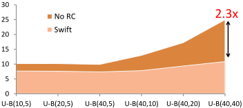
| Alg. | Bur | Hur | U-B(20,10) | U-B(40,20) |
|---|---|---|---|---|
| Running Time (s): Swift v.s. Static Dep | ||||
| Static Dep | 0.986 | 1.642 | 4.433 | 7.722 |
| Swift | 0.988 | 1.492 | 3.891 | 4.514 |
| Speedup | 0.998 | 1.100 | 1.139 | 1.711 |
| Calls to Likelihood Functions | ||||
| Static Dep | 1▷8 ⇤ 107 | 2▷7 ⇤ 107 | 1▷5 ⇤ 108 | 3▷0 ⇤ 108 |
| Swift | 1▷8 ⇤ 107 | 1▷7 ⇤ 107 | 4▷1 ⇤ 107 | 5▷5 ⇤ 107 |
| Calls Saved | 0% | 37.6% | 72.8% | 81.7% |
In Tab. 3, "Swift" is up to 1.7x faster than "Static Dep", thanks to up to 81% reduction of likelihood function evaluations. Note that for the model with fixed dependencies (Bur), the overhead by ACU is almost negligible: 0▷2% due to traversing the hashmap to access to child variables.
5.3 Swift against other PPL systems
We compare Swift with other systems using LW, PMH and Gibbs respectively on the benchmark models. The running time is presented in Tab. 4. The speedup is measured between Swift and the fastest one among the rest. An empty entry means that the corresponding PPL fails to perform inference on that model. Though these PPLs have different host languages (C++, Java, Scala, etc.), the performance difference resulting from host languages is within a factor of 2 3 .
5.4 Experiment on real-world dataset
We use Swift with Gibbs to handle the probabilistic principal component analysis (PPCA) [Tipping and Bishop, 1999], with real-world data: 5958 images of digit "2" from the handwritten digits dataset (MNIST) [LeCun et al., 1998]. We compute 10 principal components for the digits. The training and testing sets include 5958 and 1032 images respectively, each with 28x28 pixels and pixel value rescaled to [0↪ 1].
Since most benchmark PPL systems are too slow to handle this amount of data, we compare Swift against other two Speedup 12 1 1 -
3 http://benchmarksgame.alioth.debian.org/
| PPL | Bur | Hur | U-B (20,10) | T-K | GMM | 1-GMM |
|---|---|---|---|---|---|---|
| LWwith 106 samples | ||||||
| Church | 9.6 | 22.9 | 179 | 57.4 | 1627 | 1038 |
| Figaro | 15.8 | 24.7 | 176 | 48.6 | 997 | 235 |
| BLOG | 8.4 | 11.9 | 189 | 49.5 | 998 | 261 |
| Swift | 0.04 | 0.08 | 0.54 | 0.24 | 6.8 | 1.1 |
| Speedup | 196 | 145 | 326 | 202 | 147 | 214 |
| PMH with 106 samples | ||||||
| Church | 12.7 | 25.2 | 246 | 173 | 3703 | 1057 |
| Figaro | 10.6 | - | 59.6 | 17.4 | 151 | 62.2 |
| BLOG | 6.7 | 18.5 | 30.4 | 38.7 | 72.5 | 68.3 |
| Swift | 0.11 | 0.15 | 0.4 | 0.32 | 0.76 | 0.60 |
| Speedup | 61 | 121 | 75 | 54 | 95 | 103 |
| Gibbs with 106 samples | ||||||
| BUGS | 87.7 | - | - | - | 84.4 | - |
| Infer.NET | 1.5 | - | - | - | 77.8 | - |
| Swift | 0.12 | 0.19 | 0.34 | - | 0.42 | 0.86 |
| Speedup | 12 | - | 185 | |||
185 1
Table 4: Running time (s) of Swift and other PPLs on the benchmark models using LW, PMH and Gibbs.
scalable PPLs, Infer.NET and Stan, on this model. Both PPLs have compiled inference and are widely used for real-world applications. Stan uses HMC as its inference algorithm. For Infer.NET, we select variational message passing algorithm (VMP), which is Infer.NET's primary focus. Note that HMC and VMP are usually favored for fast convergence.
Stan requires a tuning process before it can produce samples. We ran Stan with 0, 5 and 9 tuning steps respectively 4 . We measure the perplexity of the generated samples over test images w.r.t. the running time in Fig. 6, where we also visualize the produced principal components. For Infer.NET, we consider the mean of the approximation distribution.
Swift quickly generates visually meaningful outputs with around 105 Gibbs iterations in 5 seconds. Infer.NET takes 13.4 seconds to finish the first iteration 5 and converges to a result with the same perplexity after 25 iterations and 150 seconds. The overall convergence of Gibbs w.r.t. the running time significantly benefits from the speedup by Swift.
For Stan, its no-U-turn sampler [Homan and Gelman, 2014] suffers from significant parameter tuning issues. We also tried to manually tune the parameters, which does not help much. Nevertheless, Stan does work for the simplified PPCA model with 1-dimensional data. Although further investigation is still needed, we conjecture that Stan is very sensitive to its parameters in high-dimensional cases. Lastly, this experiment also suggests that those parameter-robust inference engines, such as Swift with Gibbs and Infer.NET with VMP, would be preferred at practice when possible.
4 We also ran Stan with 50 and 100 tuning steps, which took more than 3 days to finish 130 iterations (including tuning). However, the results are almost the same as that with 9 tuning steps.
5 Gibbs by Swift samples a single variable while Infer.NET processes all the variables per iteration.
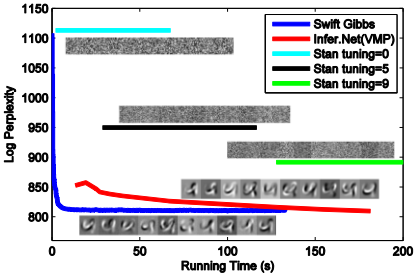
6 Conclusion and FutureWork
We have developed Swift, a PPL compiler that generates model-specific target code for performing inference. Swift uses a dynamic slicing framework for open-universe models to incrementally maintain the dependency structure at runtime. In addition, we carefully design data structures in the target code to avoid dynamic memory allocations when possible. Our experiments show that Swift achieves orders of magnitudes speedup against other PPL engines.
The next step for Swift is to support more algorithms, such as SMC [Wood et al., 2014], as well as more samplers, such as the block sampler for (nearly) deterministic dependencies [Li et al., 2013]. Although FIDS is a general framework that can be naturally extended to these cases, there are still implementation details to be studied.
Another direction is partial evaluation, which allows the compiler to reason about the input program to simplify it. Shah et al. [2016] proposes a partial evaluation framework for the inference code (PI in Fig. 1). It is very interesting to extend this work to the whole Swift pipeline.
Acknowledgement
We would like to thank our anonymous reviewers, as well as Rohin Shah for valuable discussions. This work is supported by the DARPA PPAML program, contract FA875014-C-0011.
@inproceedings{ijcai2016p512,
  title     = {Swift: Compiled Inference for Probabilistic Programming Languages},
  author    = {Wu, Yi and Li, Lei and Russell, Stuart J. and Bodík, Rastislav},
  booktitle = {Proceedings of the Twenty-Fifth International Joint Conference on
               Artificial Intelligence, {IJCAI-16}},
  publisher = {AAAI Press / International Joint Conferences on Artificial Intelligence},
  editor    = {Subbarao Kambhampati},
  pages     = {3637--3644},
  year      = {2016},
  month     = {7},
  url       = {https://ijcai.org/proceedings/2016/512},
}
TY - CPAPER TI - Swift: Compiled Inference for Probabilistic Programming Languages AU - Wu, Yi AU - Li, Lei AU - Russell, Stuart J. AU - Bodík, Rastislav T2 - Proceedings of the Twenty-Fifth International Joint Conference on Artificial Intelligence, IJCAI-16 PB - AAAI Press / International Joint Conferences on Artificial Intelligence PY - 2016 SP - 3637 EP - 3644 UR - https://ijcai.org/proceedings/2016/512 ER -Copied
Machine-readable versions of this paper, for tools and AI agents:





