
Efficient Algorithms for Spanning Tree Centrality
Proceedings of the Twenty-Fifth International Joint Conference on Artificial Intelligence. Pages 3733-3738.
Abstract
In a connected graph, spanning tree centralities of a vertex and an edge measure how crucial they are for the graph to be connected. In this paper, we propose efficient algorithms for estimating spanning tree centralities with theoretical guarantees on their accuracy. We experimentally demonstrate that our methods are orders of magnitude faster than previous methods. Then, we propose a novel centrality notion of a vertex, called aggregated spanning tree centrality, which also considers the number of connected components obtained by removing the vertex. We also give an efficient algorithm for estimating aggregated spanning tree centrality. Finally, we experimentally show that those spanning tree centralities are useful to identify vulnerable edges and vertices in infrastructure networks.
- [Anthonisse, 1971] J M Anthonisse. The rush in a directed graph. Stichting Mathematisch Centrum. Mathematische Besliskunde, (BN 9/71):1-10, 1971.
- [Barrat et al., 2008] A. Barrat, M. Barthélemy, and A. Vespignani. Dynamical processes on complex networks. Cambridge University Press, Cambridge, MA, 2008.
- [Bavelas, 1950] Alex Bavelas. Communication patterns in task-oriented groups. The Journal of the Acoustical Soci- ety of America, 22(6):725-730, 1950.
- [Bernstein et al., 2014] Andrey Bernstein, Daniel Bienstock, David Hay, M Uzunoglu, and Gil Zussman. Power grid vulnerability to geographically correlated failures -analy- sis and control implications. In INFOCOM, pages 2634- 2642, 2014.
- [Burton and Pemantle, 1993] R Burton and R Pemantle. Lo- cal characteristics, entropy and limit theorems for span- ning trees and domino tilings via transfer-impedances. The Annals of Probability, 21:1329-1371, 1993.
- [Freeman, 1977] Linton C Freeman. A set of measures of centrality based on betweenness. Sociometry, 40(1):35, 1977.
- [Girvan and Newman, 2002] M Girvan and M E J New- man. Community structure in social and biological net- works. Proceedings of the National Academy of Sciences, 99(12):7821-7826, 2002.
- [Johnson and Lindenstrauss, 1984] W B Johnson and J Lin- denstrauss. Extensions of Lipschitz mappings into a hilbert space. Contemporary Mathematics, 26(189):189- 206, 1984.
- [Katz, 1953] Leo Katz. A new status index derived from so- ciometric analysis. Psychometrika, 18(1):39-43, 1953.
- [Kelner et al., 2014] Jonathan A Kelner, Yin Tat Lee, Lorenzo Orecchia, and Aaron Sidford. An almost-linear- time algorithm for approximate max flow in undirected graphs, and its multicommodity generalizations. In SODA, pages 217-226, 2014.
- [Kempe et al., 2003] David Kempe, Jon Kleinberg, and Éva Tardos. Maximizing the spread of influence through a so- cial network. In KDD, pages 137-146, 2003.
- [Koutis et al., 2011] Ioannis Koutis, Gary L Miller, and David Tolliver. Combinatorial preconditioners and mul- tilevel solvers for problems in computer vision and image processing. Computer Vision and Image Understanding, 115(12):1638-1646, 2011.
- [Leskovec and Krevl, 2014] Jure Leskovec and Andrej Krevl. SNAP Datasets: Stanford large network dataset collection. http://snap.stanford.edu/data, 2014. Link
- [Lovász, 1993] L Lovász. Random walks on graphs: A sur- vey. Combinatorics, Paul Erdős is eighty, 2(1):1-46, 1993.
- [Lusseau et al., 2003] D. Lusseau, K. Schneider, O. J. Bois- seau, P. Haase, E. Slooten, and S. M. Dawson. The bot- tlenose dolphin community of Doubtful Sound features a large proportion of long-lasting associations. Behavioral Ecology and Sociobiology, 54:396-405, 2003.
- [Mavroforakis et al., 2015] Charalampos Mavroforakis, Richard Garcia-Lebron, Ioannis Koutis, and Evimaria Terzi. Spanning edge centrality: Large-scale computation and applications. In WWW, pages 732-742, 2015.
- [Newman and Girvan, 2004] M Newman and M Girvan. Finding and evaluating community structure in networks. Physical Review E, 69(2):026113, 2004.
- [Pagani and Aiello, 2013] G A Pagani and M Aiello. The power grid as a complex network: a survey. Physica A: Statistical Mechanics and its Applications, 392(11):2688- 2700, 2013.
- [Panconesi and Srinivasan, 2006] Alessandro Panconesi and Aravind Srinivasan. Randomized distributed edge coloring via an extension of the chernoff-hoeffding bounds. SIAM Journal on Computing, 26(2):350-368, 2006.
- [Qi et al., 2015] Xingqin Qi, Edgar Fuller, Rong Luo, and Cun-quan Zhang. A novel centrality method for weighted networks based on the kirchhoff polynomial. Pattern Recognition Letters, 58:51-60, 2015.
- [Spielman and Srivastava, 2011] Daniel A Spielman and Nikhil Srivastava. Graph sparsification by effective resis- tances. SIAM Journal on Computing, 40(6):1913-1926, 2011.
- [Teixeira et al., 2013] A S Teixeira, P T Monteiro, J A Carric ¸o, M Ramirez, and A P Francisco. Spanning edge betweenness. In Workshop on Mining and Learning with Graphs, pages 27-31, 2013.
- [Wilson, 1996] David Bruce Wilson. Generating random spanning trees more quickly than the cover time. In STOC, pages 296-303, 1996.
References were extracted automatically from the PDF and may contain errors.
Full text extracted automatically from the PDF; figures, tables and equations may differ. The PDF is the version of record.
Introduction
Measuring the importance of edges and vertices is a fundamental task in network analysis. Many importance notions have been proposed in the literature such as degree centrality, betweenness centrality [Anthonisse, 1971; Freeman, 1977], closeness centrality [Bavelas, 1950], and Katz centrality [Katz, 1953], and they are used in various applications such as community detection [Girvan and Newman, 2002; Newman and Girvan, 2004], suppressing the epidemics [Barrat et al., 2008], and maximizing the spread of influence [Kempe et al., 2003].
Among those centralities, in this paper, we focus on spanning tree centrality [Teixeira et al., 2013; Qi et al., 2015]. In a connected graph G = (V↪ E), the spanning tree centrality of an edge e 2 E is defined as the probability that e is used in a uniformly sampled spanning tree. Although the spanning tree centrality was originally used to reconstruct a phylogenetic tree from evolutionary relations among species [Teixeira et al., 2013], it turns out that it measures how crucial an edge is for the graph to be connected. Similar centrality notion for vertices was also introduced in [Qi et al., 2015].
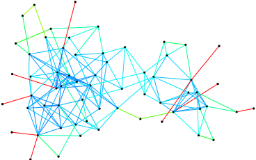
To get intuition, we depicted spanning tree centralities of edges in a social network formed by bottlenose dolphins [Lusseau et al., 2003] in Figure 1. We can observe that edges on the periphery have high spanning tree centralities because the network will be disconnected by removing a few of those edges. On the other hand, edges in the middle of a community has a small spanning tree centrality because there are many paths bypassing them, and hence they can be safely removed without disconnecting the graph.
Spanning tree centrality is a useful notion for identifying vulnerable edges and vertices. For example, infrastructure networks such as power grids should be robust against physical attacks and natural disasters, and it is important to maintain its connectivity so that all the users can access the infrastructure [Bernstein et al., 2014; Pagani and Aiello, 2013]. Spanning tree centrality directly measures how edges and vertices are important to keep the graph connected. Also, it is reported that edges of high spanning tree centralities are important for disseminating information through a social network [Mavroforakis et al., 2015].
Although several exact and approximation methods have been proposed for computing spanning tree centralities [Teixeira et al., 2013; Mavroforakis et al., 2015; Qi et al., 2015], those methods are not scalable enough to find vulnerable edges and vertices in large real-world networks, and resolving this issue is the main motivation of this paper.
Our Contributions
In this paper, we propose efficient algorithms for estimating spanning tree centrality with theoretical guarantees on their accuracy. Our algorithms sample spanning trees uniformly at random sufficiently many times using Wilson's algorithm [Wilson, 1996], and then estimate the spanning tree centralities of edges or vertices using those samples. Combined with several speeding-up techniques, our algorithms run orders of magnitude faster than previous methods on realworld networks. Because of the efficiency of our methods, we can now identify vulnerable edges and vertices in large networks. Then, we experimentally show that protecting edges and vertices of high spanning tree centralities makes a power grid network robust against random failures of edges and vertices.
The effect of vertex failures in infrastructure networks is often assessed by the resulting number of connected components [Bernstein et al., 2014]. We introduce a novel notion, called aggregated spanning tree centrality, which measures the importance of vertices with respect to this criteria. Then, we give an efficient algorithm for estimating aggregated spanning tree centrality with theoretical guarantee on its accuracy. Using a power grid network, we experimentally show that the failures of vertices with high aggregated spanning tree centralities indeed result in a large number of connected components compared to other centrality notions.
Related Work
The notion of spanning tree centrality for edges was introduced in [Teixeira et al., 2013] for reconstructing a phylogenetic tree from evolutionary relationships among species. Their exact method is based on Kirchhoff's matrix-tree theorem and computes determinants of matrices polynomially many times. This makes their algorithm slow, and it can only handle graphs of tens of thousands of edges within an hour.
An approximation algorithm based on dimension reduction through the Johnson-Lindenstraus lemma [Johnson and Lindenstrauss, 1984] was proposed by [Spielman and Srivastava, 2011]. A more practical version of this algorithm was given by [Mavroforakis et al., 2015]. Their algorithm uses an almost linear-time algorithm for solving symmetric diagonally dominant (SDD) systems [Koutis et al., 2011]. Despite these sophisticated techniques, their algorithm can only handle graphs of million edges within an hour. We will experimentally show that our algorithms can accurately estimate spanning tree centrality on graphs of millions of edges within a minute.
Spanning tree centrality for vertices was introduced in [Qi et al., 2015]. Their method is also an exact method based on Kirchhoff's matrix-tree theorem and hence impractical.
A spanning centrality of an edge is often called effective resistance as it corresponds to effective resistance when we regard a graph as an electrical circuit. See [Lov´asz, 1993] for consequences of this interpretation and connections with random walk. Theoretically, the spanning tree centrality of an edge can be well approximated in almost linear time [Spielman and Srivastava, 2011] and is used as a building block of designing almost linear time algorithms for other problems such as spectral sparsifier construction [Spielman and Srivastava, 2011] and approximate maximum flow [Kelner et al., 2014].
Preliminaries
In this section, we introduce basic notions used throughout this paper and review several concentration inequalities.
For an integer k 2 N, [k] denotes the set ¶1↪ 2↪ ▷ ▷ ▷ ↪ k♦. For a↪ b 2 R and ✏ > 0, a = b ◦ ✏ means b - ✏ a b + ✏. For a probabilistic event X, [X] denotes its indicator, that is, [X] = 1 if X holds and 0 otherwise.
Let G = (V↪E) be a graph. For a vertex v 2 V , dG(v) denotes the degree of v. For a set of vertices S ✓ V , G[S] denotes the subgraph of G induced by S.
We call an edge a bridge if the number of connected components increases by removing it. Similarly, we call a vertex an articulation point if the number of connected components increases by removing it. A graph is called biconnected if it does not have any articulation point. A biconnected component of a graph is its maximal biconnected subgraph.
Symbols n and m will denote the number of vertices and edges, respectively, of the input graph.
Spanning Tree Centrality
Let G = (V↪ E) be a connected graph. We define θG as the uniform distribution over spanning trees of G. By T ⇠ θG, we mean that we sample a spanning tree T from θG. We introduce three kinds of spanning tree centralities, one for edges and the other two for vertices.
Definition 1 (Teixeira et al. 2013). Let G = (V↪E) be a connected graph. The spanning tree centrality of an edge e 2 E, denoted by stG(e), is defined as PrT⇠θG [e 2 T ].
Definition 3. Let G = (V↪ E) be a connected graph. The aggregated spanning tree centrality of a vertex v 2 V , denoted by astG(v), is defined as ET⇠θG [dT (v)].
Definition 2 (Qi et al. 2015). Let G = (V↪ E) be a connected graph. The spanning tree centrality of a vertex v 2 V , denoted by stG(v), is defined as PrT⇠θG [dT (v) ≥ 2].
We omit subscripts when they are clear from the context. Below, we explain intuitions behind those definitions.
The spanning tree centrality of an edge measures how it is like a bridge. Indeed, if an edge e = (u↪ v) is a bridge, then e is used in any spanning tree and hence st(e) = 1. On the other hand, if there are many other paths between u and v that bypass e, then e is unlikely used in a uniformly sampled spanning tree, and hence st(e) will be small.
The spanning tree centrality of a vertex measures how it is like an articulation point. Indeed, if a vertex v is an articulation point, then v cannot be a leaf in a spanning tree and hence st(v) = 1. On the other hand, if v is contained in a tightly connected community and is not an articulation point, then st(v) becomes small. For example, if v is a vertex in a complete graph of n vertices, then by Kirchhoff's matrix tree theorem, we can easily show that st(v) = 1-(1-1◁n)n-2 ! 1 - 1◁e (n ! 1).
The aggregated spanning tree centrality of a vertex incorporates the number of connected components obtained by removing the vertex. To see this, note that ast(v) = P1i=1 PrT⇠θG [dT (v) ≥ i]. Here, PrT⇠θG [dT (v) ≥ i] can be seen as a generalization of st(v) in the sense that it measures how v is like an articulation point such that the number of connected components increases by at least i - 1 by removing v.
Concentration Inequalities
We will use following Hoeffding's inequality in our analysis.
Lemma 4. Let X1↪ ▷ ▷ ▷ ↪ Xq be independent random variables in [0↪ 1] and X = Pi2[q] Xi. Then for any 0 < ✏ < 1, we have
We say that random variables X1↪ ▷ ▷ ▷ ↪Xq are negatively correlated if Pr[Vi2[q] Xi] Qi2[q] Pr[Xi]. Even when random variables are dependent, if they are negatively correlated, then the following concentration inequality holds:
Lemma 5 (Panconesi and Srinivasan 2006). Let X1↪ ▷ ▷ ▷ ↪Xq be random variables in ¶0↪ 1♦ that are negatively correlated and X = Pi2[q] Xi. Then for any 0 < ✏ < 1, we have
For an edge e 2 E, let Xe be the indicator corresponding to the event that e is used in a spanning tree sampled from θG. Then, we have the following fact.
Lemma 6 (Burton and Pemantle 1993). Let G = (V↪E) be a connected graph. Random variables ¶Xe♦e2F for any F ✓ E are negatively correlated.
Hence, we can apply Lemma 5 to the set ¶Xe♦e2F for any set of edges F ✓ E.
Algorithms
In this section, we explain our algorithms for estimating spanning tree centralities.
Spanning Tree Centrality of Edges
Our algorithm for estimating spanning tree centralities of edges is based on Wilson's algorithm [Wilson, 1996], which samples a spanning tree uniformly at random. We need several notions to explain Wilson's algorithm.
Let G = (V↪ E) be a graph and P = (v1↪ ▷ ▷ ▷ ↪ v`) be a path in G, that is, ¶vi↪ vi+1♦ 2 E for each i 2 [`-1]. We define the loop erasure of P, denoted by LE(P), as the path obtained from P by removing cycles. More formally, we define indices ij inductively using the following rule: i1 = 1 and ij+1 = max¶i 2 [`] : vi = vij ♦ + 1. The induction stops when we have vij = v` for the current j. Let `0 be the last index j for which ij is defined. Then, LE(P) is defined as the path (vi1 ↪ ▷ ▷ ▷ ↪ vi`0 ).
Wilson's algorithm is given in Algorithm 1. It takes a graph G = (V↪E) and a vertex r 2 V , called the root, as its input. Let v1↪ ▷ ▷ ▷ ↪ vn-1 be an arbitrary ordering of V ∩¶r♦. We start with a tree T consisting of a single vertex r. Then, for each
Algorithm 1 Wilson's algorithm
- 1: procedure WILSON(G, r)
- 2: T the tree consisting of a single vertex r.
- 3: Let v1↪ ▷ ▷ ▷ ↪ vn-1 be an arbitrary ordering of V ∩ ¶r♦.
- 5: Let P be a random walk from vi to T .
- 4: for i = 1 to n - 1 do
- 6: Add the loop erasure LE(P) to T .
- 7: return T .
Algorithm 2 Spanning Tree Centrality for Edges
- 1: procedure ST-EDGE(G↪ r↪ ✏↪ δ)
- 2: q dlog(2m◁δ)◁(2✏2 )e.
- 3: for i = 1 to q do
- 4: Ti WILSON(G, r).
- 5: for each e 2 E do
- 7: return ¶e st(e)♦e2E .
- 6: e st(e) 1q Pi2[q] [e 2 Ti].
i 2 [n-1], we perform a random walk from vi until it reaches some vertex in T , and then add to T the loop erasure LE(P) of the obtained random walk P. Note that, if vi is already a vertex in T , then P is a walk consisting of a single vertex vi, and hence T does not change. It is clear that Wilson's algorithm always returns a spanning tree when G is connected. Indeed the following holds.
Theorem 7 (Wilson 1996). For a connected graph G = (V↪E) and a vertex r 2 V , WILSON(G↪ r) uniformly samples a spanning tree of G. The expected running time is Pu2V ∩¶r♦ ⇡G(u)G(u↪ r).
Here, ⇡G(u) denotes the probability of staying at a vertex u 2 V in the stationary distribution of a random walk on G, and G(u↪ v) denotes the commute time between two vertices u↪ v 2 V , that is, the expected number of steps in a random walk starting at u, before v is visited and then u is reached again. Note that ⇡G(u) = dG(u)◁2m, where m is the number of edges, as we consider undirected connected graph.
The choice of the root r and the vertex ordering v1↪ ▷ ▷ ▷ ↪ vn-1 much affect the practical performance. We will discuss several strategies later.
With the aid of Wilson's algorithm, we can efficiently estimate spanning edge centralities of edges by sampling a sufficient number of spanning trees and then counting how many of them use a particular edge (Algorithm 2). We have the following guarantee on its accuracy and time complexity:
Theorem 8. Let G = (V↪E) be a connected graph, r 2 V be a vertex, and 0 < ✏↪ δ < 1. With probability at least 1 - δ, ST-EDGE(G↪ r↪ ✏↪ δ) outputs ¶e st(e)♦e2E with e st(e) = st(e) ◦ ✏ for every e 2 E. The expected running time is dlog(2m◁δ)◁(2✏2 )e · Pu2V ⇡G(u)G(u↪ r).
Proof. By Hoeffding's inequality, for each edge e 2 E, the probability that e st(e) = st(e) ◦ ✏ holds is at least 1 - δ◁m. By union bound, the probability that e st(e) = st(e) ◦ ✏ holds for every e 2 E is at least 1 - δ. The time complexity is immediate from Theorem 7.
Algorithm 3 Spanning Tree Centrality for Vertices
- 1: procedure ST-VERTEX(G↪ r↪ ✏↪ δ)
- 2: q dlog(2n◁δ)◁(2✏2 )e.
- 3: for i = 1 to q do
- 4: Ti WILSON(G, r).
- 5: for each u 2 V do
- 7: return ¶e st(u)♦u2V .
- 6: e st(u) 1q Pi2[q] [dTi (u) ≥ 2].
Algorithm 4 Aggregated Spanning Tree Centrality
- 1: procedure AST-VERTEX(G↪ r↪ ✏↪ δ)
- 2: ✏0 e⇥(✏◁ log(n◁δ)). (e⇥(·) hides the log factor.)
- 3: q e⇥(log(n◁δ)◁✏02 ). 4: for i = 1 to q do 5: Ti WILSON(G, r).
- 6: for each u 2 V do
- 8: return ¶f ast(u)♦u2V .
- 7: f ast(u) 1q Pi2[q] dTi (u).
We will see that, in real-world networks, most edges have large spanning tree centralities, say, more than 0▷1. Hence, we can detect important edges by choosing ✏ a small constant, that is, a value independent of the graph size.
Spanning Tree Centrality of Vertices
Our algorithm for estimating spanning tree centralities of vertices is very similar to the one for edges (Algorithm 3). We have the following guarantee:
Theorem 9. Let G = (V↪E) be a connected graph, r 2 V be a vertex, and ✏↪ δ > 0. Then with probability at least 1 - δ, ST-VERTEX(G↪ r↪ ✏↪ δ) outputs ¶e st(u)♦u2V with e st(u) = st(u) ◦ ✏ for every u 2 V . The expected running time is dlog(2n◁δ)◁(2✏2 )e · Pu2V ⇡G(u)G(u↪ r).
As the proof of Theorem 9 is quite similar to that of Theorem 8, we omit the details.
Aggregated Spanning Tree Centrality of Vertices
In this section, we explain our algorithm for estimating aggregated spanning tree centralities of vertices. Our algorithm is given in Algorithm 4. It simply samples a sufficient number of spanning trees, and then computes the average degree of each vertex in those spanning trees.
If we simply apply Hoeffding's inequality, then we can only guarantee that, with high probability, f ast(u) approximates ast(u) to within ✏dG(u) for every u 2 V . We want a stronger guarantee because ast(u) is typically much smaller than dG(u). To this end, we use the fact that edges in a uniformly sampled spanning tree are negatively correlated, and we get the following guarantee:
Theorem 10. Let G = (V↪E) be a connected graph, r 2 V be a vertex, and ✏↪ δ > 0. Then with probability at least 1 - δ, AST-VERTEX(G↪ r↪ ✏↪ δ) outputs ¶f ast(u)♦u2V with f ast(u) = ast(u) ◦ (✏(1 + ast(u)) + δ) for every u 2 V . The expected running time is eO(log3 (n◁δ)◁✏2 · Pu2V ⇡G(u)G(u↪ r)).
Proof. We fix a vertex u 2 V . We show that the algorithm outputs f ast(u) with f ast(u) = ast(u) ◦ (✏(1 + ast(u)) + δ) with probability 1 - δ◁n. Then, the first claim follows by union bound.
Let Yi = dTi (u) for each i 2 [q]. Let N ≥ ast(u) be a parameter determined later, and we define Yi↪N = Yi · [Yi N] and Yi↪>N = Yi · [Yi > N] for each i 2 [q]. Note that Yi = Yi↪N + Yi↪>N holds. Hence, f ast(u) = 1q Pi Yi = 1q Pi Yi↪N + 1q Pi Yi↪>N holds. By Hoeffding's bound,
holds with probability at least 1 - δ◁(2n).
Let ✏00 = N◁ast(u)-1. Note that ✏00 ≥ 0 because we chose N ≥ ast(u). For any i 2 [q], by Lemma 5, we have
By choosing N = max¶2e · ast(u)↪ log(2qn◁δ)♦, the probability of having Yi > N becomes at most δ◁(2qn). Then by union bound, with probability at least 1 - δ◁(2n), we have Yi N for every i 2 [q]. In other words, Yi↪>N = 0 for every i 2 [q].
Since Yi n, we have E[Yi↪>N ] n · δ◁(2qn) = δ◁(2q), which means that E[Yi↪N ] = ast(u)-E[Yi↪>N ] ≥ ast(u)- δ◁(2q). Also, it is clear that E[Yi↪N] = ast(u)-E[Yi↪>N] ast(u).
Combining arguments above, with probability at least 1 - δ◁n, we have
By choosing ✏0 = ✏◁(2e log(2qn◁δ)), we have f ast(u) = ast(u) ◦ (δ + ✏(1 + ast(u))). Note that the dependency between ✏0 and q is cyclic because we need q = ⇥(log(n◁δ)◁✏02 ). However, this recurrence has a solution ✏0 = e⇥(✏◁ log(n◁δ)) and q = e⇥(log(n◁δ)◁✏2 ). The analysis of the time complexity is obvious.
Speeding-up techniques
In this section, we discuss several techniques for speeding up our algorithms.
Biconnected-component decomposition
Let G = (V↪E) be a connected graph. Suppose that biconnected components C1↪ ▷ ▷ ▷ ↪ Ck are attached at an articulation point u 2 V . Then, we can uniformly sample a spanning tree T of G by uniformly sampling spanning trees T1↪ ▷ ▷ ▷ ↪ Tk of G[C1]↪ ▷ ▷ ▷ ↪G[Ck], respectively, and attaching them at u. This means that stG(e) = stG[Ci](e) for any edge e 2 G[Ci]. Hence, it suffices to process smaller graphs G[C1]↪ ▷ ▷ ▷ ↪ G[Ck] separately.
[Mavroforakis et al., 2015] proposed to reduce the input graph to its 2-core, a maximal subgraph of the minimum degree at least two. Our decomposition technique surpasses the reduction to the 2-core because after splitting the graph at articulation points, we get bridges and biconnected components, which are subgraphs of the 2-core.
Vertex ordering
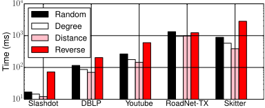
We consider the following strategies for the vertex ordering strategies used in Wilson's algorithm: Random, Degree, Distance, and Reverse. In the first three strategies, we choose a vertex with the highest degree as the root. Other vertices are randomly shuffled, sorted in decreasing order of degrees, and sorted in increasing order of distances from the root in Random, Degree, and Distance, respectively. In Reverse, a vertex with the lowest degree is chosen as the root and other vertices are sorted in increasing order of degrees.
Experiments
In this section, we demonstrate the efficiency of our methods and the effectiveness of spanning tree centralities for finding vulnerable edges and vertices in real-world networks.
Environment All the proposedmethods were implemented in C++11 and compiled with gcc 4.8.3 with -O3 option. Unless stated otherwise, we used biconnected-component decomposition and Distance strategy for vertex ordering. The implementation of the algorithm proposed by [Mavroforakis et al., 2015], which we refer to the MGKT algorithm, was obtained from authors' website 1 . All experiments were conducted with a single thread on a Linux server with Intel Xeon X5675 3.07GHz CPU and 288GB Memory.
Datasets We conducted all experiments on real-world social, road, and infrastructure networks. All datasets used in our experiments can be downloaded from Stanford Network Analysis Project [Leskovec and Krevl, 2014]. Table 1 shows the information of datasets.
Spanning Tree Sampling Performance
We first evaluate the runtime of sampling spanning trees with our speed-up techniques. Note that the runtime of our centrality estimation algorithms is dominated by the time for sampling spanning trees. Therefore, the overall running time is easily obtained by multiplying the time for sampling a spanning tree and the number of required spanning trees, which is determined by the error parameter ✏.
Speed-up by the biconnected-component decomposition
Table 2 shows the average runtime of sampling a spanning tree, where we sampled 1,000 spanning trees in total. Note that we can sample a spanning trees in less than 2 seconds on Orkut, which is a large social network with over one million edges. Biconnected components decomposition consistently reduces the runtime of sampling a spanning tree. In particular, we can sample spanning trees more than 40% faster on sparse networks such as DBLP and Youtube.
1 http://cs-people.bu.edu/cmav/centralities
| Dataset | n | m | n0 | m0 | STe |
|---|---|---|---|---|---|
| US-PowerGrid | 4.9K | 6.6K | 3.0K | 4.6K | 0.77 |
| Gnutella | 63K | 148K | 34K | 119K | 0.20 |
| Epinions | 76K | 509K | 36K | 365K | 0.17 |
| Slashdot | 77K | 905K | 47K | 439K | 0.13 |
| DBLP | 426K | 1.0M | 211K | 884K | 0.60 |
| Youtube | 1.2M | 3.0M | 452K | 2.3M | 1.00 |
| RoadNet-TX | 1.4M | 1.9M | 1.1M | 1.6M | 1.00 |
| Skitter | 1.7M | 11M | 1.4M | 11M | 1.00 |
| Pokec | 1.6M | 22M | 1.5M | 22M | 1.00 |
| Orkut | 3.1M | 117M | 3.0M | 117M | 0.51 |
| Dataset | TG | TBC | TBC◁TG |
|---|---|---|---|
| DBLP | 132.1 | 78.7 | 0.60 |
| Youtube | 297.1 | 133.1 | 0.45 |
| RoadNet-TX | 1288.2 | 997.9 | 0.77 |
| Skitter | 494.0 | 371.2 | 0.75 |
| Pokec | 652.0 | 574.5 | 0.88 |
| Orkut | 1462.9 | 1380.6 | 0.94 |
Vertex ordering strategies
We examined how vertex ordering strategies affect the efficiency of sampling spanning trees. Figure 2 shows the average runtime for each strategy to sample a spanning tree, where we sampled 1,000 spanning trees in total. We can observe that Distance is the fastest among the four strategies on almost all datasets. Apparently, this is because we can avoid long unnecessary random walks in the early stage of Wilson's algorithm by starting random walks from vertices close to the root.
Edge Centrality Estimation Performance
Among the three spanning tree centralities, we take the spanning tree centrality for edges as an example, and compare our method with the previous MGKT algorithm. We obtained similar results for other centralities.
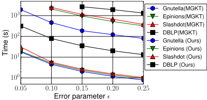
We compare the runtime of our method and the MGKT algorithm on several small networks. We chose the failure probability δ = 1◁n. For an error parameter ✏, our method samples dlog(2m◁δ)◁(2✏2 )e spanning trees and guarantees e st(e) = st(e)◦✏ for every edge with probability at least 1-δ and the MGKT algorithm guarantees (1-✏)2 st(e) e st(e) (1+✏)2 st(e) for every edge with probability at least 1-δ. We cannot directly compare those algorithms because our method guarantees absolute error whereas the MGKT algorithm guarantees relative error. However, as shown in Table 1, the important edges have large centrality values, say, more than 0.1, and hence we can claim that our method with ✏ = 0▷05 gives a sufficient accuracy in comparison with the MGKT algorithm with ✏ = 0▷25. Under this setting, our method runs orders of magnitude faster than the MGKT algorithm as shown in Figure 3.
Effectiveness of Spanning Tree Centralities
We now demonstrate the effectiveness of (aggregated) spanning tree centralities of edges and vertices.
Connectivity
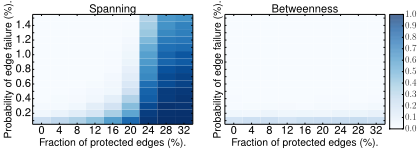
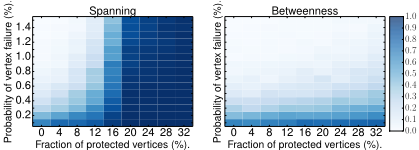
We first show that, using US-PowerGrid, which is a realworld infrastructure network, spanning tree centralities of edges/vertices are useful to identify important edges/vertices for maintaining connectivity. In our experiments, we protected a certain fraction of edges/vertices with the highest centrality values in terms of spanning tree centrality or betweenness centrality, and removed each unprotected edge/vertex with a certain probability. Then, we examined the probability that the network remained connected. The results are shown in Figure 4 and 5. We can see that show spanning tree centrality is a better measure for identifying important edges and vertices to maintain connectivity.
Number of connected components
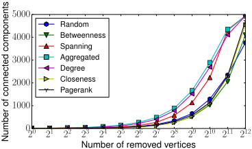
Finally, we examine the effectiveness of aggregated spanning tree centrality by considering the number of connected components. For clarity, this time, instead of protecting vertices, we removed vertices from the ones with higher centrality values. Figure 6 illustrates the result. We used the largest connected component of US-PowerGrid as the initial graph. For each different centrality measure, we removed the vertices with highest centrality values from the graph, and then computed the numbers of connected components. Larger resulting numbers of connected components mean that removed vertices are key vertices to connect many different parts of the graph. From Figure 6, we clearly see that our aggregated spanning tree centrality performs best in this experiment.
Conclusions
In this paper, we gave efficient algorithms for estimating spanning tree centrality. Our algorithms are orders of magnitude faster than previous methods. By experiment, we confirmed that spanning tree centralities are to identify vulnerable edges and vertices in infrastructure networks.
Acknowledgments
T. H., T. A., and Y. Y. are supported by JST, ERATO, Kawarabayashi Large Graph Project. T. A. is supported by JSPS Grant-in-Aid for Research Activity Start-up (No. 15H06828) and PRESTO, JST. Y. Y. is supported by JSPS Grant-in-Aid for Young Scientists (B) (No. 26730009), MEXT Grant-in-Aid for Scientific Research on Innovative Areas (No. 24106003).
@inproceedings{ijcai2016p525,
  title     = {Efficient Algorithms for Spanning Tree Centrality},
  author    = {Hayashi, Takanori and Akiba, Takuya and Yoshida, Yuichi},
  booktitle = {Proceedings of the Twenty-Fifth International Joint Conference on
               Artificial Intelligence, {IJCAI-16}},
  publisher = {AAAI Press / International Joint Conferences on Artificial Intelligence},
  editor    = {Subbarao Kambhampati},
  pages     = {3733--3738},
  year      = {2016},
  month     = {7},
  url       = {https://ijcai.org/proceedings/2016/525},
}
TY - CPAPER TI - Efficient Algorithms for Spanning Tree Centrality AU - Hayashi, Takanori AU - Akiba, Takuya AU - Yoshida, Yuichi T2 - Proceedings of the Twenty-Fifth International Joint Conference on Artificial Intelligence, IJCAI-16 PB - AAAI Press / International Joint Conferences on Artificial Intelligence PY - 2016 SP - 3733 EP - 3738 UR - https://ijcai.org/proceedings/2016/525 ER -Copied
Machine-readable versions of this paper, for tools and AI agents:





