
Identifying Key Observers to Find Popular Information in Advance
Proceedings of the Twenty-Fifth International Joint Conference on Artificial Intelligence. Pages 3761-3766.
Abstract
Identifying soon-to-be-popular items in web services offers important benefits. We attempt to identify users who can find prospective popular items. Such visionary users are called observers. By adding observers to a favorite user list, they act to find popular items in advance. To identify efficient observers, we propose a feature selection based framework. This uses a classifier to predict item popularity, where the input features are a set of users who adopted an item before others. By training the classifier with sparse and non-negative constraints, observers are extracted as users whose parameters take a non-zero value. In experiments, we test our approach using real social bookmark datasets. The results demonstrate that our approach can find popular items in advance more effectively than baseline methods.
- [Armentano et al., 2013] Marcelo Gabriel Armentano, Daniela Godoy, and Analía A Amandi. Followee rec- ommendation based on text analysis of micro-blogging activity. Information systems, 38(8):1116-1127, 2013.
- [Bottou, 1998] Léon Bottou. Online algorithms and stochas- tic approximations. In David Saad, editor, Online Learn- ing and Neural Networks. Cambridge University Press, Cambridge, UK, 1998. revised, oct 2012.
- [Du et al., 2013] Nan Du, Le Song, Hyenkyun Woo, and Hongyuan Zha. Uncover topic-sensitive information dif- fusion networks. In Proceedings of the Sixteenth Interna- tional Conference on Artificial Intelligence and Statistics, pages 229-237, 2013.
- [Duchi et al., 2011] John Duchi, Elad Hazan, and Yoram Singer. Adaptive subgradient methods for online learning and stochastic optimization. JMLR, 12:2121-2159, 2011.
- [Garcia-Herranz et al., 2014] Manuel Garcia-Herranz, Este- ban Moro, Manuel Cebrian, Nicholas A. Christakis, and James H. Fowler. Using friends as sensors to detect global- scale contagious outbreaks. PLoS ONE, 9(4):e92413, 04 2014.
- [Gomez Rodriguez et al., 2013] Manuel Gomez Rodriguez, Jure Leskovec, and Bernhard Schölkopf. Structure and dy- namics of information pathways in online media. In Pro- ceedings of the 6th ACM International Conference on Web Search and Data Mining, pages 23-32. ACM, 2013.
- [Hannon et al., 2011] John Hannon, Kevin McCarthy, and Barry Smyth. Finding useful users on twitter: twit- tomender the followee recommender. In Advances in In- formation Retrieval, pages 784-787. Springer, 2011.
- [Iwata et al., 2013] Tomoharu Iwata, Amar Shah, and Zoubin Ghahramani. Discovering latent influence in on- line social activities via shared cascade poisson processes. In Proceedings of the 19th ACM SIGKDD International Conference on Knowledge Discovery and Data Mining, pages 266-274. ACM, 2013.
- [Kong et al., 2014] S Kong, F Ye, and L Feng. Predicting future retweet counts in a microblog. Journal of Compu- tational Information Systems, 10(4):1393-1404, 2014.
- [Kupavskii et al., 2012] Andrey Kupavskii, Liudmila Os- troumova, Alexey Umnov, Svyatoslav Usachev, Pavel Serdyukov, Gleb Gusev, and Andrey Kustarev. Prediction of retweet cascade size over time. In Proceedings of the 21st ACM International Conference on Information and Knowledge Management, pages 2335-2338. ACM, 2012.
- [Li et al., 2014] Yang Li, Yiheng Chen, Ting Liu, and Wen- chao Deng. Predicting the popularity of messages on micro-blog services. In Social Media Processing, pages 44-54. Springer, 2014.
- [Menjo and Yoshikawa, 2008] Takashi Menjo and Masatoshi Yoshikawa. Trend prediction in social bookmark service using time series of bookmarks. In Proceedings of WWW2008 Workshop on Social Search and Mining, 2008.
- [Pinto et al., 2012] Pedro C Pinto, Patrick Thiran, and Mar- tin Vetterli. Locating the source of diffusion in large-scale networks. Physical Review Letters, 109(6):068702, 2012.
- [Tang and Yang, 2010] Xuning Tang and Christopher C Yang. Identifing influential users in an online healthcare social network. In IEEE International Conference on In- telligence and Security Informatics, pages 43-48. IEEE, 2010.
- [Trusov et al., 2010] Michael Trusov, Anand V Bodapati, and Randolph E Bucklin. Determining influential users in Internet social networks. Journal of Marketing Research, 47(4):643-658, 2010.
- [Wetzker et al., 2008] Robert Wetzker, Carsten Zimmer- mann, and Christian Bauckhage. Analyzing social book- marking systems: A del.icio.us cookbook. In ECAI 2008 Mining Social Data Workshop, pages 26-30, 2008.
- [Xiao, 2010] Lin Xiao. Dual averaging methods for regular- ized stochastic learning and online optimization. JMLR, 11:2543-2596, 2010.
- [Ying et al., 2012] Josh Jia-Ching Ying, Eric Hsueh-Chan Lu, and Vincent S Tseng. Followee recommendation in asymmetrical location-based social networks. In Proceed- ings of the 2012 ACM Conference on Ubiquitous Comput- ing, pages 988-995. ACM, 2012.
- [Yu and Kak, 2012] Sheng Yu and Subhash Kak. A survey of prediction using social media. CoRR, abs/1207.0016, 2012.
- [Zaman et al., 2010] Tauhid R. Zaman, Ralf Herbrich, Jur- gen Van Gael, and David Stern. Predicting information spreading in Twitter. In Proceedings of NIPS2010 Work- shop on Computational Social Science and the Wisdom of Crowds, 2010.
References were extracted automatically from the PDF and may contain errors.
Full text extracted automatically from the PDF; figures, tables and equations may differ. The PDF is the version of record.
1 Introduction
Users in web services often share their favored or adopted items, such as messages (e.g. Twitter), web pages (Reddit), images/movies (Instagram), products (Amazon), and local services (Yelp). When a user finds a favorite item in the social networking services (SNSs), he/she adopts it, for example, by bookmarking a web page in a social bookmarking site or by retweeting on Twitter. Also, when a user purchases a product via an e-commerce website, he/she sometimes submits the review of this product, which is accessible online.
The early detection of popular items is beneficial for anyone. For example, it helps a company to make the plan of marketing strategies effective [Yu and Kak, 2012]. Or it helps a researcher to identify prospective research topics before other teams. Or it helps a gourmet to make a reservation at a hidden fine restaurant before it gets crowded.
To obtain popular items in advance, we investigate the task of identifying observers that are early adopters of popular items. Although the majority of users knows popular information after becoming a trend, some users may find it before it starts trending. Such special users would be experts who know the items more than others, heavy users who constantly monitor information, prescient users who have good insight for the future, or influential people whose choices influence those of other users. If such users are recruited to a favorite user list, they can help identify likely future trends.
Identifying observers provides more benefits than the approaches that merely predict popular items such as previous works [Kupavskii et al., 2012; Li et al., 2014; Kong et al., 2014]. It can easily personalize the obtained items by changing observers: if an observer has different preferences with us, we should remove him/her in our favorite user list. Also, when the followed observers are special users as described above, we will acquire expert knowledge from their activities. For example, their reviews in e-commerce websites give insight for finding out good products by ourselves.
Selecting appropriate observers from the massive number of users is a hard task. If inefficient observers are selected, an excessive number of items will be collected, and identified popular items will be swamped by many unpopular items. Also, if the selected observers are late majority, the most of obtained items will have become popular, and the first-mover advantage will be lost. One solution is to apply the methods for estimating influential users on SNSs [Trusov et al., 2010; Tang and Yang, 2010]. However, these methods suppose that the network among users is given. Such user network does not often exist in web services such as e-commerce.
To identify efficient observers, we take an approach based on feature selection in machine learning. We use a classifier to predict whether a given item would become popular or not in the future. The input features are users who adopted the item in advance. By training the classifier with sparse and non-negative constraints, only parameters of users who frequently adopted popular items in advance take a non-zero value. We then select the users as observers. Moreover, for augmenting the effective number of training samples, we design the loss function as an expectation over the time evolving of adoptions, which is solved by stochastic optimization. Our approach only uses event data: an event is an adoption by a user for an item with a time stamp. Such event log can be obtained from many web services, and the approach will be more widely applicable than user network based methods.
2 ProblemFormulation
Suppose we seek to extract observers who can find prospective popular items but avoid selecting unpopular ones. More rigorously, we specify two requirements for the adoption behavior of observers as follows: (a) they adopt a s-popular item-the item that is in top s percent in terms of the number of adoptions 1 -before (b) m users adopt that item. The possible values of s and m depend on the data. We exclude at least some extreme values, e.g. s = 100. Figure 1 gives examples of the adoption behavior that either satisfies or fails to satisfy these requirements. The right hand side of the figure represents time-popularity curves of items A and B. The upper horizontal line means the threshold of s-popularity. Thus, item A is s-popular, and item B is not s-popular. The lower line shows the threshold of users adopting the items more or less than m times. The adoption behavior of user 1 satisfies (a) but not (b): he/she adopts popular item A, but m users have adopted it. The adoption behavior of user 2 satisfies (b) but not (a): he/she adopts item B before m users adopt it, but item B fails to become s-popular. The adoption behavior of user 3 satisfies both (a) and (b).
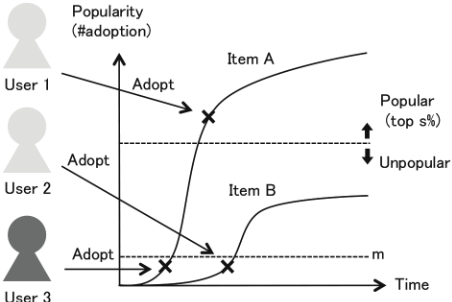
Suppose we have an event log E = ¶(ie↪ ue↪ te)♦♣E♣ e=1 , where (ie↪ ue↪ te) denotes the eth event that user ue 2 U adopts item ie 2 I at time te T. I is a set of items, U is a set of users, and T is the period of the event log. The event log E enables us to know whether each adoption satisfies (a) and (b) or not. Using this data, we extract the observers O ⇢ U whose adoptions frequently satisfy (a) and (b).
3 ProposedMethods
3.1 Item classification by popularity
For our task, we use a binary classifier that divides items into popular and unpopular ones. Let yi 2 ¶0↪ 1♦ be a binary target variable that takes one when item i is popular, and zero otherwise. The input features of the classifier indicate users who adopt the item. Let xi = (xi↪0↪ xi↪1↪ ▷ ▷ ▷ ↪ xi↪♣U♣) be a (♣U♣ + 1)-dimensional input feature vector. The first element is defined as xi↪0 = 1, which is introduced in the feature vector to represent a bias term conveniently. The value xi↪u for 1↪ ▷ ▷ ▷ ↪ ♣U♣ is defined as follows:
1 We assume that adoption occurs at most once for each (user, item) pair and users do not undo adoption.
where mi↪u 2 ¶0↪ 1↪ ▷ ▷ ▷ ↪ ♣U♣ - 1♦ is the ranking of user u adopting item i, and m is a threshold. mi↪u takes 0 when user u is ranked first for item i. The set of feature-target pairs ¶(xi↪ yi)♦♣I♣ i=1 represents requirements (a) and (b) from Section 2 and is derived from the event log E.
As the classifier, we employ logistic regression with L1 regularization and non-negative constraints for weight parameters. The loss function of logistic regression is given by:
where
σ(·) is the sigmoid function,w = (w0↪w1↪ ▷ ▷ ▷ ↪w♣U♣) is the (♣U♣+1)-dimensional weight parameter vector, and w0 is the bias parameter. Under the regularization and constraints, the optimum solution w⇤ is obtained via the following minimization problem:
where ˆw = (w1↪ ▷ ▷ ▷ ↪ w♣U♣) is the weight parameter vector except for bias w0, R( ˆw) = λ♣♣ ˆw♣♣1 is the L1 regularized term, and λ > 0 is the regularized parameter. R♣U♣ ≥0 denotes ♣U♣- dimensional space on non-negative real numbers, constraining the possible values of ˆw on non-negative space.
The non-negative constraints and L1 regularization for ˆw help for selecting observers. Without the non-negativity, the classifier would give negative weights for users who frequently adopt unpopular items. Although this will improve prediction performance, this does not serve the purpose of feature selection; we are not interested in such "novice" observers. L1 regularization makes w⇤ sparse, which means it eliminates weak or redundant observers.
3.2 Augmenting temporal information
In (2), we have ♣I♣ training samples where each feature vector has m non-zero elements. However, the setting of m is somewhat arbitrary. For instance, by changing m to 1↪ ▷ ▷ ▷ ↪ ♣U♣, we obtain ♣U♣ different training datasets. These "padded" samples contain richer information than the original samples, and will improve the performance. From this intuition, we introduce feature vector xi(z) = (xi↪0(z)↪ xi↪1(z)↪ ▷ ▷ ▷ ↪ xi↪♣U♣(z)) with varying thresholds, where each element xi↪u(z) for 1↪ ▷ ▷ ▷ ↪ ♣U♣ is defined as follows:
Here, z > 0 is the real-valued varying threshold. As in xi↪0, the first element is defined as xi↪0(z) = 1. If the number of events (i.e. adoptions) in item i was Ei, xi(z) can represent Ei different feature vectors. The event log E can have at most ♣E♣ different training samples, which is greater than ♣I♣.
The training samples with high threshold values z would not be important for our task because these samples include information of late adoptions. In contrast, samples with low threshold values would be important because they only include information of early adoptions. To take into account these importance, we introduce p(z) as the probability density function over threshold z. By weighting all possible training samples with p(z), the augmented loss is derived as the expectation of ` with respect to z:
As a result, the problem is written as follows:
Note that this data augmented method (7) includes the above non-augmented method (4) as the special case of setting p(z) = δ(z -m) where δ(·) is the delta function.
Before solving (7), we need to choose p(z). Because the optimal p(z) may be different for each dataset, we prepare some flexible distribution and determine its parameters by cross validation. In the experiments, we used the Weibull distribution of which the density is given by:
where k is a shape parameter, and ✓ is a scale parameter. 2 The Weibull distribution includes the exponential distribution (k = 1) and the Rayleigh distribution (k = 2) as a special case. It can also represent heavy/right tailed distribution.
3.3 Learning algorithm
Unfortunately, (7) may not be solved by standard optimization methods such as gradient descent because the expectation is not analytically written. The expectation is, however, approximated by many samples ¶zs♦Ss=1 as follows:
On the basis of the approximation, we consider solving (7) with stochastic optimization. Note that because both ` and R are convex, general stochastic optimization algorithms such as stochastic gradient descent are guaranteed to converge to w⇤ [Bottou, 1998].
We use the regularized dual averaging method with the adaptive gradient method (Ada-RDA) [Xiao, 2010; Duchi et al., 2011]. Ada-RDA repeatedly selects one sample randomly and updates the parameters for many times. A feature-target pair (xi(z)↪ yi) is sampled, where i is randomly drawn from
2 In contrast to (5), z in the Weibull distribution can take 0. However, this will be not a serious problem as explained in Section 3.3.
¶1↪ 2↪ ▷▷▷↪ ♣I♣♦, and z is drawn from the probability distribution having the density p(z). At the nth step, the Ada-RDA updates the parameter w by using the current weight vector wn = (wn↪0↪ ▷ ▷ ▷ ↪ wn↪♣U♣), as follows:
where
sign(·) is the sign function, [·]+ is the hinge function, and ⌘ > 0 and ✏ ≥ 0 are learning parameters. gn↪u is the uth element of a gradient vector gn with respect to w at nth step. Note that the outer [·]+ in (10) ensures the non-negativity of wn+1↪u, and the bias termwn+1↪0 is updated without the regularization and the non-negative constraint. The whole learning algorithm is shown as Algorithm 1. In this paper, we set the number of epochs to C and repeat the updates C times for the item set I. "shuffle(I)" returns the randomly aligned index set of items. "z ⇠ p(z)" means that z is drawn from the distribution having the density p(z). We set p(z) to (8) in our experiments. 3 If we set p(z) = δ(z -m), Algorithm 1 is also employed for the learning of the non-augmented method (4). After C♣I♣ iterations, we obtain the learned parameter w⇤ . Finally, we extract observers O from the learned w⇤ as follows:
One problem of this method is that it can not specify the number of observers in advance. A method to address this problem is grid search of λ. If we want to obtain d observers, we can search them by repeating the learning algorithm for some prepared λs. However, grid search does not ensure that just d observers are always obtained.
This problem also arises in a more general case: extracting D sets of observers ¶Od♦Dd=1 , where Od denotes the set of observers consisting of d users. Extracting some sets with different sizes in advance is practically useful for quick responses to users of our method. Grid search of λ also suffers from obtaining ¶Od♦Dd=1 completely; grid search would often fail to obtain some sets in ¶Od♦Dd=1 .
To address this problem, we consider interpolating the set of observers by a larger one. Suppose we want to obtain Od but only have Od0 where d0 > d. The smaller elements in the learned w⇤ for Od0 are less influential in the classifier, and the corresponding users would be also less effective. Thus,
3 As noted above, z in the Weibull distribution can take 0. However, the probability that z takes just 0 is 0, and thus the effect would be almost ignored. When z takes 0, the sampled feature is "empty"; this means all users take 0. While our experiments did not exclude this empty feature, we would be also able to ignore the feature.
Algorithm 1 Ada-RDA (E, λ, ⌘, ✏)
1: Input: E = ¶(ie↪ ue↪ te)♦♣E♣ e=1 , λ, ⌘, ✏ 2: Initialize: w1 = 0, n = 1 3: for epoch c = 1↪ ▷ ▷ ▷ ↪C do 4: ¶i0s ♦♣I♣ s=1 = shuffle(I) 5: for i = i01 ↪ ▷ ▷ ▷ ↪ i0♣I♣ do 6: z ⇠ p(z) 7: Set yi and xi(z) according to (5) 8: Compute gn according to (12) 9: Compute gn and hn according to (11) 10: Compute wn+1 according to (10) 11: n = n + 1 12: end for 13: end for 14: Output: w⇤ =wnOd0 after removing d0 - d users taking smaller values would give a good approximation of Od.
Based on this insight, we perform a forward backward algorithm to extract D sets of observers. The algorithm is given as Algorithm 2. We prepare λ = ¶λj♦Jj=1 , which is sorted in descending order. 4 This indicates that the larger index j (i.e. smaller λj) are used, the more non-zero elements the learned w⇤ tends to have. In lines 5 to 20, the algorithm repeats extracting and storing observers by forward grid search of λ. If D or more observers were obtained, the algorithm finishes the grid search. Next, the algorithm performs backward interpolation of missing sets of observers (lines 21 to 27). "remove(w, r)" in line 24 returns a vector in which the smaller non-zero r elements in w are replaced by zero. If Od is empty, the algorithm interpolates it with the larger and non-empty set Od+1. Finally, the algorithm outputs ¶Od♦Dd=1 without the missing sets.
4 RelatedWork
Methods for predicting the number of adoptions in SNSs have been proposed before [Kupavskii et al., 2012; Li et al., 2014; Kong et al., 2014], and attempts have been made to improve predictive performance. In contrast with earlier approaches, our proposed method uses classifiers to identify observers who can adopt popular items in advance.
In most of existing user or followee recommendation methods, these suggest users who have similar preference to obtain personalized information [Hannon et al., 2011; Armentano et al., 2013; Ying et al., 2012]. A similar method for locating the sources of information diffusion in social networks has been also proposed [Pinto et al., 2012]. Our aim of obtaining popular information in advance is different.
Algorithms for social network inference have been proposed [Du et al., 2013; Iwata et al., 2013; Gomez Rodriguez et al., 2013; Zaman et al., 2010]. By simulating information diffusion on inferred networks, item popularity could be
4 Algorithm 2 supposes that λJ learns the weight vector that has D or more non-zero elements.
Algorithm 2 Forward-backward extraction (E, λ, ⌘, ✏)
1: Input: E = ¶(ie↪ ue↪ te)♦♣E♣ e=1 , λ = ¶λj♦Jj=1 , ⌘, ✏ 2: Initialize: 3: Od = ;, for d = 1↪ ▷ ▷ ▷ ↪D+1 4: wd = 0, for d = 1↪ ▷ ▷ ▷ ↪D+1 5: for j = 1↪ ▷ ▷ ▷ ↪ J do 6: wj =Ada-RDA (E, λj, ⌘, ✏) 7: d = ♣observers(wj)♣ 8: if 0 < d < D and Od = ; then 9: wd = wj 10: Od = observers(wd) 11: else if d = D then 12: wD = wj 13: OD = observers(wD) 14: break 15: else if d > D then 16: wD+1 = wj 17: OD+1 = observers(wD+1) 18: break 19: end if 20: end for 21: for d =D↪ ▷ ▷ ▷ ↪ 1 do 22: if Od = ; then 23: r = ♣observers(wd+1)♣ - ♣observers(wd)♣ 24: wd = remove(wd+1, r) 25: Od = observers(wd) 26: end if 27: end for 28: Output: ¶Od♦Dd=1predicted. However, inferring networks is a challenging task as the number of unknown parameters to be estimated is the square of the number of users. In contrast, the number of unknown parameters in our proposed method is the number of users, which is more tractable. In addition, our proposed method directly learns classifiers for predicting popularity using log data, which leads to better predictive performance.
Our proposed method can be seen as a method for finding influential users. Identifying such users leads to detection of popular items as soon as possible: once those influential users adopt an item, many other users are likely to adopt the same item. There are some existing methods for detecting influential users [Trusov et al., 2010; Tang and Yang, 2010]. Garcia-Herranz et al. showed that even randomly selected users are helpful for detecting outbreaks on Twitter [GarciaHerranz et al., 2014]. However, these methods need to user network, which is unavailable in many web services.
A closely related work is the method of [Menjo and Yoshikawa, 2008]. For predicting item popularity, this method also uses event logs. The method scores the importance of users and outputs the ranking of potential item popularity at a certain time by using the scores. Although the method seems to be able to use our problem at first glance, it does not meet our task. The method assumes each item has some growing interval that rapidly increases the number of adoptions. Then, the method gives high scores to users that adopt an item before all the growing intervals even when the item has been already popular. In contrast, we require to obtain items before becoming a trend, and thus the method is not relevant to our task.
| Dataset | #items | #users | #events |
|---|---|---|---|
| ajax | 7,924 | 9,553 | 458,706 |
| css | 11,647 | 16,528 | 955,829 |
| design | 39,100 | 33,481 | 2,015,359 |
| java | 8,703 | 6,641 | 289,976 |
| javascript | 10,841 | 11,254 | 641,639 |
| linux | 14,835 | 13,867 | 615,193 |
| news | 3,807 | 5,267 | 133,571 |
| opensource | 7,485 | 6,923 | 296,902 |
| photography | 9,910 | 11,704 | 399,751 |
| science | 4,790 | 4,505 | 130,747 |
| webdesign | 16,171 | 18,035 | 1,038,161 |
5 Experiments
To evaluate our proposed augmented and non-augmented methods, we used Delicious datasets [Wetzker et al., 2008], which comprise records of events where Delicious users bookmarked (adopted) web pages with time stamps. We used 11 datasets separated by tag information in Delicious. Users who appeared less than 30 times in every data set were excluded, and only items that were adopted more than 10 times were used. We assigned popular labels to the top s = 10 percent of items, and unpopular labels to the others. The summary of the datasets is given in Table 1.
We prepared six baseline methods. The baselines give a score to each user and select users having a high score as observers. The baselines assign the following score to user u:
Random: A random real number in [0▷0↪ 1▷0).
- Nadoptions: The number of items adopted by u.
- Nfollowers: The sum of the number of users adopting the same item as u but after u.
- Nearly: The number of times that u adopted items before m other users adopted them.
- Nearly-pos: The number of times that u adopted popular (i.e. positive) items before m other users.
- Nearly-pos/neg: Nearly-pos divided by the number of times that u adopted unpopular (i.e. negative) items before m other users.
Random and Nadoptions fail to consider requirements (a) and (b) from Section 2, because it does not take account of popularity and the order of adoptions. Nfollowers and Nearly consider (b) by giving priority to users adopting items early. However, they do not consider (a). Nearly-pos and Nearlypos/neg consider (a) and (b) by taking account of both popularity and the order of adoptions.
We did not compare any previous work described in Section 4. The methods using user network was unavailable in the Delicious datasets where the network does not exist as in many other web services. We did not also compare the methods for directly predicting popularity because the purpose is different from ours, and they require more information that is not included in the Delicious datasets. The method of [Menjo and Yoshikawa, 2008] is applicable for our experiments. However, the definition of important users and the purpose are different from ours as discussed in Section 4.
We conducted the experiments with the following settings. Items were split into ten subsets, with 90 percent of the items used as training data and the other 10 percent as test data. In the training dataset, all events were fully observed. From this training data, we extracted 100 sets of observers ¶Od♦100 d=1 using the proposed methods and the baselines respectively. In the test data, we assumed that the initial m = 10 users were only observed for each item. If several users adopted items at the same date around the threshold m, we randomly selected ten users to be observed. If at least one observer was in the initial 10 users, each method classified the item as a popular item by supposing that we could obtain the item before more than 10 other users through observers. We evaluated the methods by using the F-measure. To simplify the comparison, we computed the area under the curve (AUC) of the #observers-F-measure curve, after normalizing the axis of #observers from [1↪ 100] to [0↪ 1▷0]. We repeated the above procedure ten times while changing the training and test data (i.e. 10-fold cross validation) and took the average of the AUCs.
We set the parameters as follows. For the non-augmented method, Nearly, Nearly-pos, and Nearly-pos/neg, we set m to 10 so as to meet the above experimental setting. Although we only tested the case of m = 10, it will not be so critical for the methods; these methods are adapted according to m. The augmented and non-augmented methods are learned using Algorithm 2. We set both ⌘ and ✏ to 1▷0, and C to 20. We also set λ to the set of 500 points in [0▷00001↪ 0▷01]. For the augmented method, we needed to select the pair of parameters (k, ✓). We performed v-fold cross validation on k 2 K = ¶0▷5↪ 1▷0↪ 2▷0↪ 5▷0↪ 10▷0↪ 50▷0♦, ✓ 2 ⇥ = ¶1▷0↪ 5▷0↪ 9▷5↪ 15▷0♦, and v = 5 using training data. After computing the AUC for each fold, the pair taking the best average was used in the test. 5 Thus, the augmented method requires to validate the parameters v♣K♣♣⇥♣ times before extracting observers. However, the validation can be executed in parallel. We used 24 (= ♣K♣♣⇥♣) threads 6 in order to validate all (k, ✓)s in parallel for each fold. Note that the augmented method is closest to the non-augmented method when (k, ✓) is set to (50▷0, 9▷5). This setting ensures that the augmented method performs at least as well as the nonaugmented method.
All the results are shown in Table 2. Figure 2 illustrates the example of #observers-F-measure curve in the webdesign dataset. The results show that the augmented method had significantly better performance than the baselines for all the datasets. While both the two proposed methods had nearly equal performances for seven datasets, the augmented method was significantly better for four datasets and the average of all the datasets. This result suggests that augmentation of the training samples improves performance.
5 Some (k, ✓)s failed to obtain 100 or more observers in forward grid search of λ. Although we tried to extend the range of the grid search, the observers were not extracted. Because the performance of such (k, ✓)s was mostly poor, we ignored the (k, ✓)s and set the AUC to zero.
6 We used one server that has 16 processors and allows for computing 32 threads at a time by hyper-threading.
| Dataset | Random | Nadoptions | Nfollowers | Nearly | Nearly-pos | Nearly- pos/neg | Non-augmented | Augmented |
|---|---|---|---|---|---|---|---|---|
| ajax | 0.051 | 0.168 | 0.200 | 0.172 | 0.252 | 0.133 | 0.305 | 0.315 |
| css | 0.034 | 0.135 | 0.174 | 0.156 | 0.293 | 0.178 | 0.332 | 0.344 |
| design | 0.024 | 0.136 | 0.164 | 0.164 | 0.244 | 0.060 | 0.276 | 0.276 |
| java | 0.058 | 0.190 | 0.210 | 0.204 | 0.228 | 0.113 | 0.246 | 0.247 |
| javascript | 0.052 | 0.134 | 0.183 | 0.129 | 0.240 | 0.082 | 0.299 | 0.304 |
| linux | 0.056 | 0.171 | 0.194 | 0.195 | 0.266 | 0.102 | 0.299 | 0.298 |
| news | 0.085 | 0.163 | 0.247 | 0.224 | 0.327 | 0.306 | 0.374 | 0.376 |
| opensource | 0.082 | 0.154 | 0.177 | 0.191 | 0.235 | 0.118 | 0.255 | 0.256 |
| photography | 0.047 | 0.169 | 0.202 | 0.183 | 0.223 | 0.071 | 0.236 | 0.240 |
| science | 0.085 | 0.170 | 0.189 | 0.183 | 0.218 | 0.143 | 0.241 | 0.241 |
| webdesign | 0.034 | 0.143 | 0.168 | 0.170 | 0.291 | 0.132 | 0.336 | 0.350 |
| Average | 0.055 | 0.157 | 0.192 | 0.179 | 0.256 | 0.131 | 0.291 | 0.295 |
| Nadoptions | Nfollowers | Nearly | Nearly-pos | Nearly-pos/neg | Non-augmented | Augmented | |
|---|---|---|---|---|---|---|---|
| design | 6.00 | 16.93 | 2.57 | 4.16 | 4.15 | 118.60 | 1206.75 (1069.31) |
| webdesign | 3.18 | 10.11 | 1.24 | 2.02 | 2.02 | 28.45 | 904.02 (875.98) |
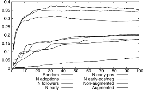
Table 3 shows the averages of runtime taken to extract observers in the design and webdesign datasets. 7 We excluded the result of Random; although it was as fast as other baselines, the performance improvement would be expected depending on the implementation. The proposed methods took more time than baselines: while baselines check training items only once, the proposed methods repeat checking them C times. The augmented method took the longest time, and the most part was used in the validation of (k, ✓). Although we computed all the (k, ✓)s in parallel, the runtime did not decrease as we expected. This is due to the overhead of the hardware scheduling and the computation of the AUC for selecting the best (k, ✓).
7 While the proposed methods were implemented by Java, baselines were done by Python.
6 Summary and Discussion
In this paper, we formulated a new problem to find observers and proposed a feature selection based framework to address the problem. Our proposed methods outperformed the baselines in real social bookmark datasets.
Let us remark the tradeoff between performance and computational cost for our proposed methods. While the augmented method outperformed the non-augmented method in many datasets, the augmented method requires additional computation caused by the cross validation of (k↪ ✓). This computation can be reduced by validating (k↪ ✓)s in parallel. If all the parameters are validated in parallel, the augmented method can run the validation ideally v♣K♣♣⇥♣ times faster. However, as described in experiments, the actual runtime will get worse than the expected one due to hardware limitation and additional costs. Thus, when setting large ♣K♣, ♣⇥♣, and v in large-scale data, we suggest using the non-augmented method. Otherwise the augmented method is recommended.
Acknowledgments
KH was supported by MEXT KAKENHI 15K16055.
@inproceedings{ijcai2016p529,
  title     = {Identifying Key Observers to Find Popular Information in Advance},
  author    = {Konishi, Takuya and Iwata, Tomoharu and Hayashi, Kohei and Kawarabayashi, Ken-ichi},
  booktitle = {Proceedings of the Twenty-Fifth International Joint Conference on
               Artificial Intelligence, {IJCAI-16}},
  publisher = {AAAI Press / International Joint Conferences on Artificial Intelligence},
  editor    = {Subbarao Kambhampati},
  pages     = {3761--3766},
  year      = {2016},
  month     = {7},
  url       = {https://ijcai.org/proceedings/2016/529},
}
TY - CPAPER TI - Identifying Key Observers to Find Popular Information in Advance AU - Konishi, Takuya AU - Iwata, Tomoharu AU - Hayashi, Kohei AU - Kawarabayashi, Ken-ichi T2 - Proceedings of the Twenty-Fifth International Joint Conference on Artificial Intelligence, IJCAI-16 PB - AAAI Press / International Joint Conferences on Artificial Intelligence PY - 2016 SP - 3761 EP - 3766 UR - https://ijcai.org/proceedings/2016/529 ER -Copied
Machine-readable versions of this paper, for tools and AI agents:





