Matching via Dimensionality Reduction for Estimation of Treatment Effects in Digital Marketing Campaigns

1 Introduction

Estimating causal treatment effects from observational (i.e., nonexperimental) data is a key problem in various fields of science [Spirtes et al., 2000; Pearl, 2009b; Morgan and Winship, 2014]. Our domain of interest is digital marketing, where a marketer has access to a collection of observational data and seeks answers to business critical questions such as whether a new advertisement attracts more clicks, whether a new campaign drives more conversions, etc. [Chan et al., 2010; Dalessandro et al., 2012; Hill et al., 2015; Barajas et al., 2015; Wang et al., 2015]. Unlike randomized experiments where the covariate distributions of the treatment and control groups are balanced in expectation, in an observational study this balance can be distorted by a confounding bias that is introduced by the systematic assignment of the treatment to the units [Rosenbaum and Rubin, 1983; Pearl, 2010; Hill and Su, 2013]. A simple and popular method to address this bias is to match the distribution of covariates in the two groups in order to create a subsample that is more balanced in the covariates [Rubin, 1973a; Stuart, 2010; Hainmueller, 2012]. The matched counterparts of the treated units in the control group are interpreted as counterfactuals, and the average treatment effect on treated (ATT) is estimated by comparing the outcomes of every matched pair.

One of the widely used matching methods is Nearest Neighbor Matching (NNM) [Rubin, 1973a]. For each treated unit, NNM finds its nearest neighbor in the control group to generate a matched pair, and the ATT is then estimated from the set of matched pairs. Different NNM methods are characterized by the choice of a distance measure for determining such a match. Some of the popularly used distance measures are Exact Matching and its variant Coarsened Exact Matching (CEM) [Iacus et al., 2011], Mahalanobis distance matching [Rubin, 1979], and Propensity Score Matching (PSM) [Rosenbaum and Rubin, 1983]. Although these estimators have been widely applied, they usually exhibit poor performance in high-dimensional data. For example, Exact Matching has to discard a lot of data in order to attain a good matching when a large set of covariates is present and hence it can result in a large bias [Rosenbaum and Rubin, 1985]. Mahalanobis distance matching uses the empirical covariance of the data, but this effectively imposes parametric assumptions on the data and therefore is prone to a bias in high dimensions [Gu and Rosenbaum, 1993]. PSM summarizes each covariate vector by a single number, namely the probability of being treated, but it also suffers from a model misspecification problem in the high-dimensional case [Caliendo and Kopeinig, 2008; King and Nielsen, 2016]. More generally, theoretical results show that the bias of a nearest-neighbor matching estimator increases with the dimensionality of the data [Abadie and Imbens, 2006], which can limit the applicability of matching estimators in real-world domains such as digital marketing.

The above motivates an approach that maintains the practical advantages of NNM while addressing its sensitivity to the high dimensionality of the data. In this work we propose a new estimator that matches the data in a low-dimensional subspace of the original space. Intuitively, a good estimator should preserve as much as possible the neighborhood relationships of the units in the input space, which motivates projections that provide guarantees of that sort. For a total number N of treated and control units, the JohnsonLindenstrauss (JL) lemma [Johnson and Lindenstrauss, 1984; Ailon and Chazelle, 2006] guarantees that a random linear projection to O(logN) dimensions preserves (withing a controllable factor) all pairwise distances of the points in the high-dimensional input space. Motivated by the JL lemma, we propose a new matching estimator that works as follows. (1) We first project the data to multiple random linear subspaces of dimension O(logN). (2) Then we estimate the treatment effect by simple nearest neighbor matching in each subspace. (3) Finally we compute the median value of the estimated effects. A theoretical treatment of the statistical properties of the new estimator is out of the scope of this paper, but we provide a careful empirical calculation of the mean square error of the estimator on semi-synthetic data, following a recently proposed experimental design that employs real data to compute statistical properties of ATT estimators [Fr¨olich et al., 2015]. As we demonstrate on semi-synthetic as well as real data from digital marketing campaigns, the proposed estimator is very robust and it consistently improves over baseline methods.

In summary, the main contributions of our work are:

• ÷ We propose the estimation of average treatment effects from observational data by means of dimensionality reduction. To the best of our knowledge, this is the first attempt to estimate treatment effects by matching in a low-dimensional subspace of the data.
• ÷ We evaluate the proposed estimator on semi-synthetic data as well as real-world data from digital marketing, and show its robustness against baseline methods. To the best of our knowledge, this is the first application of nearest-neighbor matching in the domain of digital marketing. Our approach can also be applied in other domains that involve high-dimensional observational data, such as text analysis [Roberts et al., 2015] and public health [Glass et al., 2013].

2 Background and RelatedWork

The dominant paradigm for causality in the AI literature is the structural causal model of Pearl [Pearl, 2009b], with its do(·) notation for interventions and semantics drawn from the structural equation models and graphical models for probabilistic reasoning [Spirtes et al., 2000]. A contender to the Pearl's paradigm is the counterfactual or potentialoutcome framework of Neyman-Rubin [Neyman, 1923; Rubin, 1974]. The key distinction between Pearl's framework and the counterfactual framework is that the latter allows expressing counterfactual queries as standard probabilistic queries on some probability space defined on both hypothetical and real events, subject to certain consistency constraints between the two types of events [Pearl, 2009a]. The fact that causal queries can be formulated in the familiar probability language has contributed to the popularity of the counterfactual framework for practical applications [Morgan and Winship, 2014], but the framework has also been criticized for its lack of flexibility or intuitiveness when dealing with complex settings [Pearl, 2009a]. The counterfactual framework is sufficient for demonstrating the key ideas of our work, so we have adopted it throughout.

The key assumption of the counterfactual framework is that each individual in the population of interest has a potential outcome under each (binary) treatment state, even though each individual is observed in only one treatment state at any point in time [Morgan and Winship, 2014]. More specifically, for individual (unit) i there are two possible outcomes, Yi(1) if it undergoes treatment T, and Yi(0) if it does not. The treatment effect for individual i is defined as

and one of the two terms is always missing in the data, since for each individual i we observe either Yi(1) (if i is treated) or Yi(0) (if i is in the control group). A naive idea for solving the missing data problem is to directly compare the treated and control groups. This can work if the two groups have balanced distributions, which is approximately the case in randomized trials [King and Nielsen, 2016]. In observational studies, however, the assumption of balanced distributions is unrealistic due to the systematic assignment of treatments.

The idea of matching as a method to estimate causal effects from observational data began as early as the 1940s but gained widespread attention with the work by Rubin [Rubin, 1973a; 1973b; 1974]. Since then it has been widely studied and applied in several fields of science [Stuart, 2010; Morgan and Winship, 2014]. In the methodological literature, matching is typically used as a method to form quasiexperimental contrasts by sampling comparable treatment and control cases from among two larger pools of such cases [Morgan and Winship, 2014]. Matching methods can be broadly classified into nearest neighbor matching, weighting, and subclassification. In this work we focus on Nearest Neighbor Matching (NNM): For each treated unit i, NNM finds the nearest neighbor of i in the control group in terms of a given distance measure in the covariate space, and discards the unmatched control units. The average treatment effect on the treated (ATT) is then estimated by

where NT = PNi=1 Ti is the number of treated samples, and Ti is a binary treatment indicator. Yi(1) is the observed outcome of the treated unit i, and ˆ Yi(0) is the counterfactual control outcome of unit i, which is estimated from the matched counterpart of unit i in the control group.

Early work on NNM focused on estimating the ATT when dealing with a single covariate [Rubin, 1973a; 1973b; Cochran and Rubin, 1973]. Various distance measures defining the similarity between two units while matching have been proposed in the literature. A straightforward way is to perform exact matching on the covariates, but this clearly becomes impractical when dealing with a large number of covariates or covariates containing continuous values. Mahalanobis distance matching computes the Mahalanobis distance between every pair of controlled and treated units in the covariate space and then matches the units accordingly. This is known to work well when there are relatively few covariates [Rubin, 1979], but it can fail when the number of covariates is large or when the covariates are not normally distributed [Gu and Rosenbaum, 1993].

A key development in this area was the introduction of Propensity Score Matching (PSM) [Rosenbaum and Rubin,

1983]. PSM estimates the probability of receiving treatment (aka propensity score) for each unit, without looking at the outcomes in the sample. The units are matched by simply grouping individuals with similar propensity scores, motivated by the fact that, asymptotically, at each value of the propensity score the distribution of the covariates defining the score is the same in the two groups. PSM has emerged as a very popular method for causal analysis mainly due to its simplicity [Dehejia and Wahba, 2002; Peikes et al., 2008]. However, PSM is reported to be overly sensitive to the choice of model for the propensity score [Caliendo and Kopeinig, 2008], it can increase the imbalance between the two groups [King and Nielsen, 2016], and other issues [Heckman et al., 1998; Bryson et al., 2002; King and Zeng, 2006; Pearl, 2009b].

In a key paper, Abadie and Imbens [Abadie and Imbens, 2006] analyzed the bias of NNM estimators theoretically, and found that the dimensionality of the data can have a negative effect on the bias of the estimator. In particular, they showed that the bias grows, roughly, at a rate O(N -1◁d ), where N is the sample size and d is the number of covariates. This implies that, for finite samples, the bias will increase with the dimensionality of the data. This result has motivated our approach in which matching is performed in a reduced dimension, as we describe next.

3 Randomized Nearest Neighbor Matching

Our approach hinges on the very simple idea that matching can be performed in a reduced subspace of the original covariate space. The principal motivation for such 'matching via dimensionality reduction' is a statistical one, namely to soften the dependence of the estimation bias to the data dimension [Abadie and Imbens, 2006]. As we demonstrate in the experiments section, this idea turns out to be solid.

As we are primarily interested in 'big data' applications such as digital marketing, we are constrained by computational considerations to the use of linear dimensionality reduction algorithms. Candidate algorithms here would be Principal Component Analysis (PCA) [Jolliffe, 2002], and Locality Preserving Projections (LPP) [He and Niyogi, 2004]. The LPP algorithm, in particular, aims at preserving the local neighborhood structure of the data in the embedding, and hence it seems a good choice for our problem. However, LPP relies on the choice of a kernel (that would be expensive to optimize over) and moreover it is not clear how to set the dimension of the reduced subspace. We have tried both PCA and LPP in our experiments, and we report the results in the next section.

Since we are aiming at a purely nonparametric approach, a natural choice for dimensionality reduction is via random projections. The technical tool we need is the JohnsonLindenstrauss (JL) lemma [Johnson and Lindenstrauss, 1984] that states that we can (linearly) project high-dimensional data onto a randomly generated subspace of suitable dimension while approximately preserving the original distances between points:

Johnson-Lindenstrauss (JL) lemma. For any 0 < ✏ < 1◁2 and x1↪ · · · ↪ xN 2 Rd , there exists a mapping f : Rd ! Rk , Algorithm 1. Randomized Nearest Neighbor Matching Input: Treated group XT 2 Rd⇥Nt Number of random projections m Control group XC 2 Rd⇥Nc Response variables YT and YC

Total sample size N

• 1: Choose the dimension of subspace k ⇡ O(logN)
• 2: for i from 1 to m
• 3: Generate a random projection Pi 2 Rd⇥k
• 4: Project XT and XC using Pi
• Z iT = P > i XT ↪ Z iC = P > i XC.
• 5: PerformNNM between Z iT and Z iC
• 6: Estimate the ATT A(i) from (2)
• 7: end for

Output: Return median(A)

It is known that the mapping f can be linear, giving rise to particularly simple algorithms for dimension reduction [Hegde et al., 2008; Maillard and Munos, 2012].

Our approach, dubbed Randomized Nearest Neighbor Matching, defines an ATT estimator by means of several random projections of the input covariates to subspaces of size O(logN) in accordance with the JL lemma. In particular, let XT 2 Rd⇥Nt and XC 2 Rd⇥Nc denote the treatment and control groups, where d is the dimensionality of data, Nt is the size of the treatment group, and Nc is the size of the control group.

The proposed estimator involves the following steps:

1) First, we construct m independent random linear projections, P1↪ · · · ↪ Pm 2 Rd⇥k , where k is chosen according to the JL lemma. Each entry in Pi is drawn from a univariate Gaussian distribution N(0↪ 1) (or other distributions [Achlioptas, 2001; Bingham and Mannila, 2001]). Each column of Pi is normalized to unit norm.

2) Second, we project XT and XC to low-dimensional subspaces using each of the generated projections. For the i-th subspace, this reads Z iT = P > i XT , Z iC = P > i XC, where Z iT and Z iT are the low-dimensional representations of XT and XC, respectively. We then perform nearest neighbor matching on Z iT and Z iC , and estimate a corresponding ATT A(i) using (2). The vector A 2 Rm⇥1 contains the estimated ATT in all m subspaces.

3) Finally, we choose the median value of the entries of the vector A as our estimate. This enhances the robustness of the estimator and is expected to reduce its total bias (an insight that was corroborated by our experiments).

The above steps are summarized in Algorithm 1. Note that, according to the JL lemma, the embedding dimension k does not depend on the original dimensionality of data. This makes the approach applicable to very high-dimensional data. Moreover, an attractive feature of random projections is that they preserve the privacy of data, which can be critical in applications such as digital marketing where the customer information is sensitive (we do not elaborate on this issue further here; see [Lindell and Omri, 2011; Ahmed et al., 2013]).

4 Experiments

In this section we empirically validate the proposed estimator on synthetic, semi-synthetic, and real-world digital marketing Campaign data.

4.1 Synthetic Dataset

The synthetic dataset is generated by following the procedures introduced in [Sun et al., 2015]. In particular, the sample size N is set to 1000, and the number of features d is set to 200. We define the following basis functions: f1(x) = -2 sin(2x), f2(x) = x2 - 1◁3, f3(x) = x - 0▷5, f4(x) = e-x - e-1 - 1, f5(x) = (x - 0▷5)2 + 2, f6(x) = Ix>0, f7(x) = e-x , f8(x) = cos(x), f9(x) = x2 , and f10(x) = x. The features x1↪ x2↪ · · · ↪ xd are drawn independently from the normal distribution N (0↪ 1). The binary treatment variable T is defined as T♣x = 1 if P5j=1 fj(xj) > 0 and T♣x = 0 otherwise. Finally, the model for generating outcome is Y ♣x↪ T ⇠ N(P5j=1 fj+5(xj)+T↪ 1). In this synthetic dataset, the first five features are correlated to the treatment and outcome, simulating a confounding effect, while the rest of the features are noisy covariates. The true causal effect (i.e., the ground truth value of ATT) in this dataset is 1.

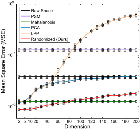
We compare our matching estimator with the following baseline methods: Raw Space (Euclidean distance), Mahalanobis, PSM, PCA, and LPP. The first two baselines match units in the high-dimensional space by using different distance measures. PSM estimates the propensity score of each unit using logistic regression, and matches units with similar scores. The latter two perform nearest neighbor matching in low-dimensional subspaces computed by PCA and LPP, respectively.

To test the quality of each estimator, we carried out the above data generation process 1000 times and we estimated the ATT for each estimator. In Figure 1 we report the mean square error (MSE) of each estimator. (The standard error is also shown as error bars). For our Randomized NNM, we set the number of random projections m to 50 (we got similar results for a wide range of values for m; results omitted.) From Figure 1 we observe that the proposed estimator achieves lower MSE than all other methods when the dimension is lower than 60. The JL bound for N = 100 is about 7, which is consistent with Figure 1; our estimator achieves the lowest MSE when the dimension varies from 5 to 10.

4.2 Digital Marketing Campaign Data

We also evaluate the performance of our estimator and baselines on a real-world digital marketing campaign dataset. The dataset contains some covariates, such as customer profile and purchase activities, which are encoded by 209dimensional binary vectors. It also includes the responses of customers to various promotions offered during the period of about one month. During this period, many campaigns were launched that involved sending promotions to customers via email, aiming at convincing the customers to purchase. In particular, several related promotions were sent to different groups of customers at about the same time. Specifically, two promotional emails were separately sent to two groups of customers, with the only difference between them being the offered discount: The first group involved offers with low discount, while the second group high discount. Due to the non-randomized (and unknown to us) assignment of promotions to customers, it is challenging to answer questions such as which promotion actually performed better than the other. Even worse, we may obtain confusing or misleading results if directly counting the average customer responses in the raw data. To see this, in the above example there were 0.8 million customers who received low discount, and 1.2 million customers who received high discount. The click response rate in the 0.8-million group was 2.24%, while this rate in the other group was only 1.16%. Without a careful causal analysis these rates could give the false impression that customers who received low discount were actually more likely to click the advertisement than those who received high discount, which is counter-intuitive and probably a wrong conclusion.

We apply matching estimators to this campaign data in order to infer the true causal effect of different promotions. Customers who received high discount promotion form the treatment group, and those with low discount form the control group. The question that we want to answer (and which is very relevant to a marketer) is whether the high discount promotion attracts more responses (e.g., open advertisements, click offers) than the low discount one. We design two empirical studies to compare the performance of our estimator against the baselines. First, we conduct a semi-synthetic experiment by virtue of pseudo-treated samples and we estimate the MSE of each estimator (here the ground truth is known). Second, we perform matching on the campaign data with real responses and we estimate the ATT (here the ground truth is unknown).

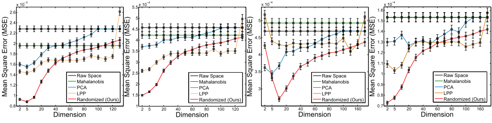
• (a) N=750, Open Response (b) N=750, Click Response (c) N=3000, Open Response (d) N=3000, Click Response

Figure 2: MSE of semi-synthetic experiment on Campaign Data. Note that the Raw Space and Mahalanobis only perform nearest matching in the original 209 dimensional data space.

Semi-synthetic Experiments

We follow the experimental design in [Fr¨olich et al., 2015] that goes as follows. First, for each treated sample (i.e., the customer who received high discount promotion), we find its nearest neighbor in the control group (i.e., customers who received low discount promotion) in terms of Euclidean distance of the covariate vectors. The treated samples are then discarded and do not play any further role in the experiment. The matched control samples form the pseudotreated 'population', and the remaining control samples form the control 'population'. Then, we repeatedly draw samples with replacement out of the 'populations', consisting of 50% pseudo-treated and 50% controlled units. Note that the true causal effect in this experiment is zero, as the pseudo-treated units did not (by default) receive any treatment.

In our experiment, the pseudo-treated 'population' contains 250,000 samples and the control 'population' contains 350,000 samples. We randomly choose subsamples from the populations for evaluation. We consider two different sample sizes, N = 750 and N = 3000, and we draw 4000 times for N = 750 and 1000 times for N = 3000 (those numbers are suggested by [Fr¨olich et al., 2015] based on theoretical arguments; we refer to their paper for details).

We considered two types of responses, open and click. The former one indicates whether a customer is attracted by the promotion, and the latter one implies a stronger incentive for purchase. We note that the responses in this campaign data are very sparse. The sparsity of open and click responses were 98.05% and 86.77%, respectively. In Figure 2 we show the MSE of different matching estimators for the two responses. We observe the following:

• ÷ Matching in the original high-dimensional space (such as Raw Space and Mahalanobis) gives poor results in general, which is consistent with the theory [Abadie and Imbens, 2006]. It validates the necessity of reducing the dimensionality of the data prior to matching.
• ÷ PCA and LPP can sometimes achieve good performance, but they are quite sensitive to the choice of reduced dimension, which makes them unstable and hence impractical for real-world applications.
• ÷ The proposed Randomized NNM estimator achieves the

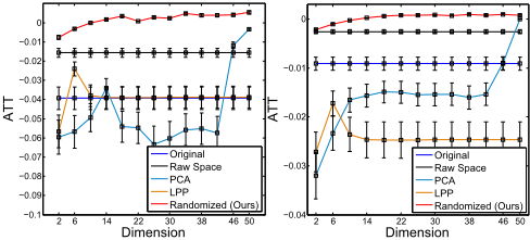
(a) N=20K, Open Response (b) N=20K, Click Response

Figure 3: ATT estimated by different methods on 20K Campaign Data. Note that the Raw Space only performs nearest matching in the original 209 dimensional data space.

lowest MSE in every case. Interestingly, the largest gap to the other methods seems to appear close to the JL bound. For example, in the case of N=3000 in the Open Response, the JL bound is log(3000) ⇡ 8, which is roughly the value at which the curve of Randomized NNM is peaked, see Figure 2(c).

Experiments on Data with Actual Treatments

Finally, we quantitatively analyze the performance of different estimators on the above campaign data using the actual treatments. That is, we estimate the causal effects of the campaign by matching the actual treated samples to the control samples. As the ground truth of the causal effect is unknown, we show the estimated ATT for Open and Click responses in Figure 3 (a) and (b), respectively. The sample size is 20,000, which consists of 8,000 treated samples and 12,000 control samples. We also examine the performance of the various estimators by drawing a larger sample set of 200,000 data points, while maintaining the ratio of treated to control samples. Figure 4 shows the results in this case. (LPP is not included because of its large computational cost on large-scale data.)

From Figure 3 and Figure 4 we observe that the original values of ATT (blue curves) are negative, which were calculated by (naively) comparing the response rates in two groups

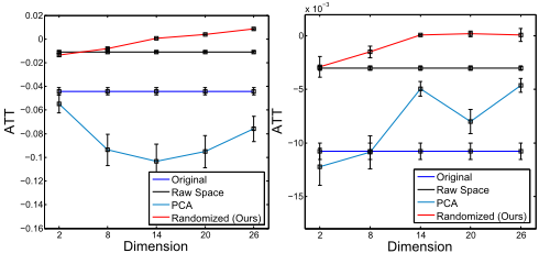
Figure 4: ATT estimated by different methods on 200K Campaign Data. Note that the Raw Space only performs nearest matching in the original 209 dimensional data space.

(see discussion in the first paragraph of this section). Such an estimated value of ATT would (wrongly) indicate that the low discount promotion is more effective than the high discount one. All the other baselines estimators also achieve negative ATT values. Only our estimator attains positive ATT, for embedding dimensions that are consistent with the JL lemma. This provides further evidence that the proposed estimator can draw meaningful causal conclusions in practice and it is robust under different settings.

5 Conclusions

We proposed a new matching estimator for estimating causal effects in digital marketing and related applications. The proposed estimator is very simple. It projects the data to several random linear subspaces, and estimates the median treatment effect by nearest-neighbor matching in each subspace. The Johnson-Lindenstrauss lemma guarantees that the neighborhood structure of the data is approximately preserved in each low-dimensional embedding, and hence matching can be done in the reduced spaces without loss. We evaluated the new estimator, as well as several baselines, on synthetic, semi-synthetic, and real-world experiments. The results attest to the quality of the proposed estimator over baseline methods.

Several important problems remain to be addressed in future work, such as dealing with the lack of common support between the treatment and control distributions [Hill and Su, 2013], identifying critical subsets of covariates [Entner et al., 2013; Silva and Evans, 2014], and dealing with highly sparse responses (e.g., purchases in digital marketing campaigns).

Acknowledgments

Part of this work was completed while the first author was an intern at Adobe Research, San Jose CA. The second author would like to thank Ricardo Silva for his feedback and for pointers to the literature. This research is supported in part by the National Science Foundation (NSF) CNS award 1314484, NSF IIS award 1449266, Office of Naval Research (ONR) award N00014-12-1-1028, ONR Young Investigator Award N00014-14-1-0484, Naval Postgraduate School (NPS)

award N00244-15-1-0041 and U.S. Army Research Office Young Investigator Award W911NF-14-1-0218, and a Research Award from Adobe.