Observability, Identifiability and Sensitivity of Vision-Aided Inertial Navigation

1 Introduction

We present a novel approach to the analysis of observability/identifiability of three-dimensional (3-D) position and orientation (termed pose) in visually-assisted navigation, whereby inertial sensors (accelerometers and gyrometers, jointly referred to as an Inertial Measurement Unit, or IMU) are used in conjunction with optical sensors (vision) to yield an estimate of the 3-D pose of the sensor platform. It is customary to frame this as a filtering problem, where the time-series of positions and orientations of the sensor platform is modeled as the state trajectory of a dynamical system, that produces sensor measurements as outputs, up to some uncertainty. Observability/identifiability analysis refers to the characterization of the set of possible state trajectories that produce the same measurements, and therefore are indistinguishable given the outputs [Soatto, 1994; Kelly and Sukhatme, 2009; Mourikis and Roumeliotis, 2007; Jones et al., 2007; Martinelli and others, 2014].

The parameters in the model are either treated as unknown constants (e.g., calibration parameters) or as random processes (e.g., accelerometer and gyro biases) and included in the state of the model, which is then driven by some kind of uninformative ("noise") input. Because noise does not affect the observability of a model, for the purpose of analysis it is usually set to zero. However, the input to the model of accelerometer and gyro bias is typically small but not independent of the state. Thus, it should be treated as an unknown input, which is known to be "small" in some sense, rather than "noise."

Our first contribution is to show that while (a prototypical model of) assisted navigation is observable in the absence of unknown inputs, it is not observable when unknown inputs are taken into account. Our second contribution is to reframe observability as a sensitivity analysis, and to show that while the set of indistinguishable trajectories is not a singleton (as it would be if the model was observable), it is nevertheless bounded. We explicitly characterize this set and bound its volume as a function of the characteristics of the inputs, which include sensor characteristics (bias rates) and the motion undergone by the platform (sufficient excitation).

Related work

In addition to the above-referenced work on visual-inertial observability, our work relates to general unknown-input observability of linear time-invariant systems addressed in [Basile and Marro, 1969; Hamano and Basile, 1983], for affine systems [Hammouri and Tmar, 2010], and non-linear systems in [Dimassi et al., 2010; Tanwani, 2011; Bezzaoucha et al., 2011]. The literature on robust filtering and robust identification is relevant, if the unknown input is treated as a disturbance. However, the form of the models involved in vision-aided navigation does not fit in the classes treated in the literature above, which motivates our analysis. The model we employ includes alignment parameters for the (unknown) pose of the inertial sensor relative to the camera.

1.1 Notation

We adopt the notation of [Murray et al., 1994], where a reference frame is represented by an orthogonal 3 ⇥ 3 positive-determinant (rotation) matrix R 2 SO(3) ▷= ¶R 2 R3⇥3 ♣ RT R = RRT = I↪ det(R) = +1♦ (the special orthogonal group) and a translation vector T 2 R3 . They are collectively indicated by g = (R↪ T) 2 SE(3) (the special Euclidean group). When g represents the change of coordinates from a reference frame "a" to another ("b"), it is indicated by gba. Then the columns of Rba are the coordinate axes of a relative to the reference frame b, and Tba is the origin of a in the reference frame b. If pa is a point relative to the reference frame a, then its representation relative to b is pb = gbapa. If Xa are the coordinates of pa, then Xb = RbaXa +Tba are the coordinates of pb. A time-varying transformation (or pose) is indicated with g(t) = (R(t)↪ T (t))

We indicate with b! a skew-symmetric matrix b! 2 so(3) ▷= ¶S 2 R3⇥3 ♣ ST = -S♦ corresponding to the cross product with the vector ! 2 R3 , so that b!v = ! ⇥ v for any vector v 2 R3 . In homogeneous coordinates, we write ¯Xb = gba ¯Xa where ¯XT = [XT 1] and ¯XT b = [(RbaXa +Tba)T 1].

1.2 MotionModel

There are several reference frames to be considered in a navigation scenario. The spatial frame s is typically attached to the Earth and oriented so that gravity γ takes the form γ T = [0 0 1]T kγk where kγk can be read from tabulates based on location and is typically around 9▷8m◁s2 . The body frame b is attached to the IMU. The camera frame c, relative to which image measurements are captured, is also unknown, although we will assume that intrinsic calibration has been performed, so that measurements on the image plane are provided in metric units [Ma et al., 2003]. The motion of a sensor platform is represented as the time-varying pose gsb of the body relative to the spatial frame.

The equations of motion (known as mechanization equations) are usually described in terms of the body frame at time t relative to the spatial frame gsb(t). Since the spatial frame is arbitrary (other than for being aligned to gravity), it is often chosen to be co-located with the body frame at time t = 0. To simplify the notation, we indicate this time-varying frame gsb(t) simply as g, and so for Rsb↪ Tsb↪ !sb↪ vsb, thus effectively omitting the subscript sb wherever it appears. This yields ˙T = v↪ ˙R = Rb!↪ ˙v = ↵↪ ˙! = w↪ ˙↵ = ⇠ where w 2 R3 is the rotational acceleration, and ⇠ 2 R3 the translational jerk (derivative of acceleration). For further details, see [Jones and Soatto, 2011].

1.3 Sensor Model

Although the acceleration ↵ defined above corresponds to neither body nor spatial acceleration, it is conveniently related to accelerometer measurements ↵imu:

| {z } where the measurement error in bracket includes a slowlyvarying mean ("bias") ↵b(t) and a residual term n↵ that is commonly modeled as a zero-mean (its mean is captured by the bias), white, homoscedastic and Gaussian noise process. In other words, it is assumed that n↵ is independent of ↵, hence uninformative. Measurements from a gyro, !imu, can be similarly modeled as

where the measurement error in bracket includes a slowlyvarying bias !b(t) and a residual "noise" n! also assumed zero-mean, white, homoscedastic and Gaussian, independent of !.

Other than the fact that the biases ↵b↪ !b change slowly, they can change arbitrarily. One can therefore consider them an unknown input to the model, or a state in the model, in which case one has to hypothesize a dynamical model for them. For instance,

for some unknown inputs wb↪ ⇠b that can be safely assumed to be small, but not (white, zero-mean and, most importantly) independent of the biases. Nevertheless, it is common to consider them to be realizations of a Brownian motion that is independent of !b↪ ↵b. This is done for convenience as one can then consider all unknown inputs as "noise." Unfortunately, however, this has implications on the analysis of the observability and identifiability of the resulting model.

1.4 Model Reduction

The equations above define a dynamical model having as output the IMUmeasurements. In this standardmodel, data from the IMU are considered as (output) measurements. However, it is customary to treat them as (known) input to the system, by writing ! in terms of !imu and ↵ in terms of ↵imu. Including the initial conditions and biases, the resulting mechanization model is

with nR = -n! and nv = -Rn↵, both typically considered independant of the state.

1.5 ImagingModel and Alignment

Initially we assume there is a collection of points Xi ↪ i = 1↪ ▷ ▷ ▷ ↪N, visible from time t = 0 to the current time t. If ⇡ : R3 ! R2 ;X 7! [X1◁X3↪ X2◁X3] is a canonical central (perspective) projection, assuming that the camera is calibrated, 1 aligned, 2 and that the spatial frame coincides with the body frame at time 0, we have

In practice, the measurements y(t) are known only up to a transformation gcb mapping the body frame to the camera, often referred to as "alignment":

Which we can add, along with the points Xis , to the state with trivial dynamics ˙gcb = 0:

1 Intrinsic calibration parameters are known.

2 The pose of the camera relative to the IMU is known.

2 Analysis of the Model

The goal here is to exploit imaging and inertial measurements to infer the sensor platform trajectory. For this problem to be well-posed, a (sufficiently exciting) realization of !imu↪ ↵imu and y should constrain the set of trajectories that satisfy (4)- (7) to be unique. If there are different trajectories that satisfy (4) with the same outputs and inputs, they are indistinguishable. If the set of indistinguishable trajectories is a singleton (contains only one element, presumably the "true" trajectory), the model (4) is observable, and one may be able to retrieve a unique point-estimate of the state using a filter, or observer.

While it is commonly accepted that the model (specifically, its equivalent reduced realization) (4), is observable, this is the case only when biases are exactly constant. But if biases are allowed to change, however slowly, the observability analysis conducted thus far cannot be used to conclude that the indistinguishable set is a singleton. Indeed, we show that this is the not the case, by computing the indistinguishable set explicitly. The following claim is proven in [Hernandez et al., 2013].

Claim 1 (Indistinguishable Trajectories) Let g(t) = (R(t)↪ T(t)) 2 SE(3) satisfy (4)-(7) for some known constant γ and functions ↵imu(t), !imu(t) and for some unknown functions ↵b(t)↪ !b(t) that are constrained to have k ˙↵b(t)k  ✏, k ˙!b(t)k  ✏, and k !b(t)k  ✏ at all t, for some ✏ < 1.

Suppose ˜ g(t) ▷= σ(gBg(t)gA) for some constant gA = (RA↪ TA), gB = (RB↪ TB), σ > 0, with bounds on the configuration space such that 3 kTAk  MA and 0 < mσ  ♣σ♣  Mσ. Then, under sufficient excitation conditions, ˜ g(t) satisfies (4)-(7) if and only if

for Ii and ki determined by the sufficient excitation conditions.

Here, sufficient excitation (m and M) refers to the nature of the motion, with more dynamic motion leading to larger values, as described in [Hernandez et al., 2013]. From these bounds, we find that the set of indistinguishable trajectories in the limit where ✏ ! 0 is parametrized by an arbitrary TB 2 R3 and rotation ✓ 2 R about gravity, termed the Gauge ambiguity, which can be explicitly fixed [Hernandez et al., 2013]. This immediately implies the following Claim 2 (unknown-input observability) The model (4)-(7) is not observable, even after fixing the Gauge ambiguity, as the indistinguishable set is not a singleton, unless biases are constant (✏ = 0) or their derivative is known exactly.

3 Here σ(g) is a scaled rigid motion: if g = (R↪ T), then σ(g) = (R↪ σT ).

We refer the reader to [Hernandez et al., 2013] for additional details and proofs, which are articulated into several steps. In practice, once the Gauge transformations are fixed, a properly designed filter can be designed to converge to a point estimate, but there is no guarantee that such an estimate coincides with the true trajectory. Instead, the estimate can deviate from the true trajectory depending on the biases. The analysis above quantifies how far from the true trajectory the estimated one can be, provided that the estimation algorithm uses bounds on the bias drift rates and the characteristics of the motion. Often these bounds are not strictly enforced but rather modeled through the driving noise covariance.

3 Empirical Validation

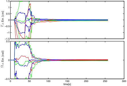
To validate the analysis, we run repeated trials to estimate the state of the platform under different motion but identical alignment (the camera is rigidly connected to the IMU) using our experimental platform [Tsotsos et al., 2015]. If alignment parameters (Tcb translational and ⌦cb parametrizing Rcb) were identifiable (or the augmented state observable), we would expect convergence to the same parameters across all trials. Instead, Fig. 1 shows that the estimates of the parameters stabilize, but to different values at each run. Nevertheless, the parameter values are in a set, whose vol1.5

1

-0.5

0 50 100 150 200 250 300 time[s] Figure 1: Convergence of alignment parameters to a set, rather than a unique point estimate, due to the lack of unknown-input observability in the presence of (realistic) non-constant biases. The mean (solid) and twice the std. dev. (dashed) of the change in estimated parameters relative to their initial nominal values across multiple trials on real data, show that different trials converge to different parameter values, but to within a bounded set.

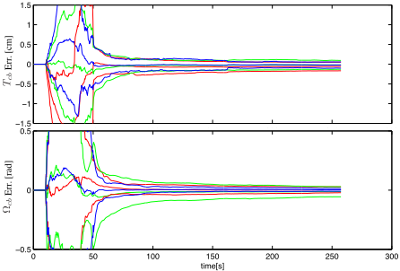
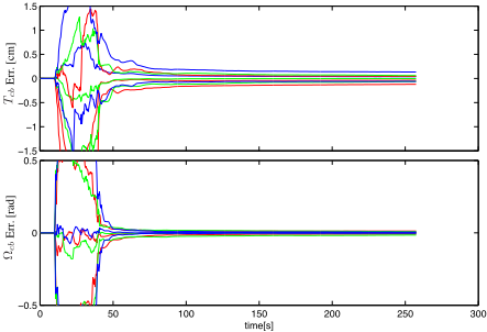
ume can be bounded based on the analysis above and the characteristics of the sensor. In particular, less stable biases, and less exciting motions, result in a larger indistinguishable set: Fig. 2 shows the same experiments with more gentle (hence less exciting) motions. Fig. 3 shows the same where

1.5

1

-0.5

0 50 100 150 200 250 300 time[s] Figure 2: The indistinguishable set is bounded depending on the characteristic of the motion. Gentler motion produces multiple trials that converge to a set of larger volume compared to Fig. 1.

the accel and gyro biases have been artificially inflated by adding a slowly time-varying offset. Additionally, we con1.5

1

-0.5

0 50 100 150 200 250 300 time[s] Figure 3: The indistinguishable set also depends on the characteristics of the sensor, and its volume is directly proportional to the sensor bias rate. Here artificial bias drift is added, resulting in a larger indistinguishable set compared to Fig. 1.

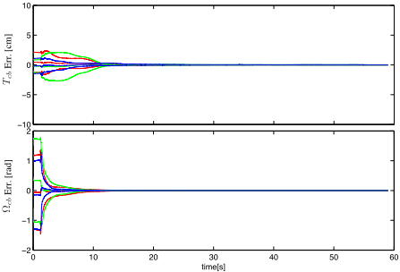
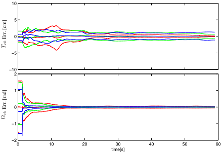
ducted Monte-Carlo experiments on the model in simulation using stationary and time-varying biases while undergoing sufficiently exciting motion. Figures 4 and 5 show the resulting estimation errors of alignment states for 50 trials each using a constant and white-noise driven bias respectively.

4 Discussion

This paper presents a overview of the analysis presented in [Hernandez et al., 2015]. We have shown that when inertial sensor biases are included as model parameters in the state of a filter used for navigation estimates, with bias rates treated as unknown inputs, the resulting model is not observable, that is, the set of indistinguishable states is not a singleton.

Consequently, we have re-formulated the problem of analyzing the convergence characteristics of (any) filters for

10

5

-2

0 10 20 30 40 50 60 time[s] Figure 4: Mean (solid line) and twice the standard deviation (dashed lines) of estimation errors of alignment parameters aggregated over 50 Monte-Carlo trials with a constant bias. 10

5

-2

0 10 20 30 40 50 60 time[s] Figure 5: Mean (solid line) and twice the standard deviation (dashed lines) of estimation errors of alignment parameters aggregated over 50 Monte-Carlo trials with a time-varying bias.

vision-aided inertial navigation not as one of observability or identifiability, but one of sensitivity, by bounding the set of indistinguishable trajectories to a set whose volume depends on motion characteristics.

The advantage of this approach, compared to the standard observability analysis based on rank conditions, is that we characterize the indistinguishable set explicitly. We quantify the "degree of unobservability" as the sensitivity of the solution set to the input; provided that sufficient-excitation conditions are satisfied, the unobservable set can be bounded and effectively be treated as a singleton. More generally, however, the analysis provides an estimate of the uncertainty surrounding the solution set, as well as a guideline on how to limit it by enforcing certain gauge transformations.

Acknowledgements

This work was supported by the Air Force Office of Scientific Research (grant no. AFOSR FA9550-12-1-0364) and the Office of Naval Research (grant no. ONR N00014-13-1-034).