The Dependence of Effective Planning Horizon on Model Accuracy

1 Introduction

When planning with Markov decision processes (MDPs), we distinguish between two different horizons (or, equivalently, discount factors). The evaluation horizon, specified by the problem formulation, is part of the definition of the ultimate measure of performance for a policy and cannot be changed. The planning horizon, on the other hand, is a parameter supplied to the planning algorithm; it affects the resulting policy but need not match the evaluation horizon. Generally, the deeper or longer the planning horizon, the greater the computational expense of computing a policy [Kearns et al., 2002; Kocsis and Szepesvari, 2006], while in principle the shallower or shorter the planning horizon (relative to the evaluation horizon), the more suboptimal the resulting policy is likely to be [Kearns et al., 2002]. Thus, there is a tradeoff between computation and optimality that is relatively well-understood in cases where the model used for planning is accurate.

⇤This paper is a condensed version of Jiang et al. [2015] and appears in IJCAI 2016 Sister Conference Best Paper Track.

In this paper, we argue that there is another important reason to use shorter planning horizons in the more realistic case where the model used for planning is estimated from data: avoiding overfitting. Specifically, we show formally that the planning horizon controls the complexity of the policy class: shorter planning horizons define less complex policy classes. As in supervised learning, the optimal complexity (and therefore the optimal planning horizon) depends on the quantity of data used to estimate the model.

2 Preliminaries: MDP planning

An MDP specifies the agent-environment interaction model as a 5-tuple M = hS↪A↪ T↪R↪ γevali, where S is the state space, A is the action space, T : S ⇥A⇥ S ! [0↪ 1] is the transition probability function, R : S⇥A ! R is the expected reward function, and γeval is the evaluation discount factor. We assume rewards are bounded in the interval [0↪Rmax]. The agent's goal is to act so as to maximize expected utility, the expected sum of future rewards discounted by γeval. A policy ⇡ : S ! A is a mapping from states to actions. A policy that maximizes expected utility in M is an optimal policy; we denote such a policy as ⇡⇤M↪γeval tomake explicit its dependence on γeval. We denote the value function of policy ⇡ evaluated in MDP M using arbitrary discount factor γ as V ⇡M↪γ 2 R♣S♣ .

Certainty-equivalence control. We are interested in the case where the model is estimated from data collected in the real world; scarcity of data then implies that our model will only be approximate. Under the principle of certaintyequivalence control we act according to the policy that is optimal for the inaccurate planning model. In particular, we will be concerned with the performance of the certainty-equivalence policy derived from an estimated model c M using a guidance discount factor γ (which might not be equal to γeval). (If c M = M and γ = γeval, the certainty-equivalence policy is optimal.) We assume c M is the maximum-likelihood model; that is, the estimated transition probability b T(s↪ a↪ s0 ) is the number of times we observe the transition (s↪ a) ! s0 in the data divided by the number of times we observe (s↪ a). (We assume that the reward function R is known in advance; see the longer version of this paper for the unknown-rewards setting [Jiang et al., 2015].) Note that our use of the certainty-equivalent policy allows us to abstract away all details of specific planning algorithms and focus solely on the influence of the guidance discount factor γ and its interaction with the quality of the M.

model c Evaluation. We emphasize that the certainty-equivalence policy computed using γ in model c M will nonetheless be evaluated in M using γeval. We capture this explicitly in our definition of the planning loss as the largest (over states) absolute difference in the values of the optimal policy ⇡⇤M↪γeval and the CE-control policy ⇡⇤c M↪γ when each is evaluated in the true environment M with the evaluation discount factor γeval. Formally, we have

where k·k1 denotes the L1 norm of a vector, i.e., the largest absolute value of any entry.

Discount factors and planning horizon. When computing a policy with guidance discount factor γ, there is an implicit notion of planning horizon. The larger γ, the longer the planning horizon, because rewards further into the future have an effect on the choice of optimal action in the current state. Indeed, in tree-search based planning algorithms such as UCT [Browne et al., 2012; Kocsis and Szepesvari, 2006], γ is explicitly translated into a planning horizon (usually 1◁(1 - γ)). Hereafter, we use guidance discount factor and planning horizon interchangeably with the understanding that the actual use depends on the nature of the planning algorithm.

Optimal guidance discount factor. The decoupling of γeval and γ is fundamental to our work. The former is specified by the MDP, while the latter is a parameter of the planning algorithm. If c M = M, the only reason for γ < γeval would be to obtain computational savings (at the expense of acting suboptimally). Our aim is to show that when c M 6=M there is another important reason to pick γ < γeval.

Given M and c M, an optimal guidance discount factor can be defined as follows:

This is the discount factor that the certainty-equivalence planner should use to minimize planning loss.

3 Planning horizon and a complexity measure

Equation 2 above suggests that γ ⇤ < γeval could be optimaland indeed this is often observed in practice-but we do not yet have clear intuitions about when or why that would be true. We offer the following explanation: γ is a complexity control parameter for certainty-equivalent planning.

3.1 A counting complexity measure

Specifically, we will show in this section that γ monotonically controls the number of policies that can be optimal for a fixed state space, action space, and reward function. When c M is estimated from a limited data set, we can therefore avoid overfitting in policy selection by restricting the number of available policies through the use of a smaller γ.

In the traditional empirical risk minimization setting for supervised learning, training data are used to evaluate the models in a given model class, and the model with the lowest training error is selected [Vapnik, 1992]. Overfitting occurs when the model class is too complex compared to the effective size of the dataset, and one way to avoid overfitting is to limit the complexity of the model class.

We draw analogies to four elements in this scenario: (1) the size of the dataset, (2) the complexity of the model class, (3) empirical risk minimization as a method for selecting a model from the class of models, and (4) some way to control model complexity. In our planning setting, the size of the dataset corresponds to the number of samples used to estimate c M. We assume that for every state-action pair (s↪ a) we observe n samples of the successor state drawn from the true transition function. (For now, we assume that the rewards R are known exactly.) The model class in our setting is the set of policies that are optimal for at least one possible c M; we refer to this as the policy class. The complexity of the model class corresponds to the size of the policy class, i.e., the number of policies that are potentially optimal. Empirical risk minimization corresponds to selecting the optimal policy for c M, as achieved by certainty-equivalence planning. These three correspondences are evident. It remains to show that reducing the guidance discount factor γ corresponds to reducing the size of the policy class searched during planning. Theorem 1 shows that this is indeed the case.

Theorem 1. For any fixed state space S, action space A, and reward function R, define the policy class

Then the following claims hold:

1. ⇧R↪γ ✓ ⇧R↪γ 0 8γ↪ γ 0 : 0  γ  γ 0 < 1
2. ∣∣⇧R↪0 ∣∣ = 1 if, for all s 2 S, argmaxa2AR(s↪ a) is unique.

The condition for claim 1 ensures that there are no ties in the maximal reward for each state, and the condition for claim 3 requires that one cannot obtain the maximal reward at every state.

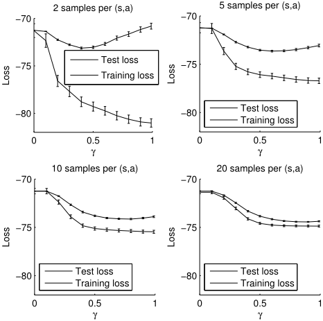
Taken together, the three claims of Theorem 1 show that γ monotonically adjusts the size of the policy class from 1 to at least ♣A♣♣S♣-2 , which is "almost all" of the ♣A♣♣S♣ possible policies. Thus the choice of guidance discount factor tightly controls complexity. Figure 1 illustrates this by showing that, as γ varies from 0 to γeval, we recover the traditional learning curves from supervised learning. Training loss decreases monotonically as γ increases, while test loss is U-shaped, indicating that an overly large γ causes overfitting. (See the caption for details on how these empirical results were produced and how training and testing loss are defined.) We can also see in Figure 1 that the location of the minimum of the test loss curve-that is, the optimal γ-shifts to the right as we receive more data.

We sketch proofs for the three claims in turn. Claim 1 is straightforward; the optimal policy does not depend on T when γ = 0, thus the policy that picks the action with the highest immediate reward is optimal. The assumption guarantees that this policy is unique.

Proof sketch of Theorem 1, claim 2. We will prove that for γ  γ 0 , ⇡ 2 ⇧R↪γ ) ⇡ 2 ⇧R↪γ 0 . Let T be a transition function for which ⇡ is optimal in hS↪A↪ T↪R↪ γi. We will construct T 0 such that ⇡ is optimal in the MDP M 0 = hS↪A↪ T 0 ↪R↪ γ 0 i. The construction is as follows: let T 0 (s↪ a↪ s0 ) = (1 - ↵)T(s↪ a↪ s0 ) + ↵I(s = s0 ) where ↵ = 1-γ◁γ 0 1-γ , and I(·) is the indicator function; that is, T 0 is a transition function where, with probability 1 - ↵, transitions behave according to T, but with probability ↵, a state simply transitions to itself. Given any policy ⇡0 : S ! A, it is straightforward to show that

Consequently, ⇡ is also optimal in M 0 and so ⇡ 2 ⇧R↪γ 0 .

Proof sketch of Theorem 1, claim 3. The proof is by construction. Let (s⇤ ↪ a⇤ ) be a state-action pair that achieves the highest reward among all state-action pairs. Let s0 be a state whose maximal reward action a0 gives reward strictly less than R(s⇤ ↪ a⇤ ). Such a state always exists under the assumption for this claim in the theorem. Consider an arbitrary policy ⇡, with the only constraints that ⇡(s⇤ ) = a⇤ and ⇡(s0 ) = a0 . Then the following transition function makes ⇡ optimal for large enough γ:

where 1(·) denotes the delta distribution. Since we constrained ⇡ in only two states, the number of such policies is ♣A♣♣S♣-2 .

3.2 Planning loss bound

Completing the connection to model class complexity in supervised learning, we show that the loss of the certaintyequivalence policy for c M is bounded, with high probability, in terms of the policy class complexity ♣⇧R↪γ♣. This is analogous to a standard generalization bound [Kearns and Vazirani, 1994], and implies that an intermediate value of γ will generally be optimal; moreover, as the amount of data (n) increases, so does the optimal γ.

Theorem 2. Let M be an MDP with non-negative rewards and evaluation discount factor γeval. Let c M be an MDP comprising the true reward function of M and a transition function estimated from n samples for each state-action pair. Then certainty-equivalence planning with c M using guidance discount factor γ  γeval has planning loss

with probability at least 1 - δ.

The proof of the theorem can be found in the longer version of this paper [Jiang et al., 2015]. The upper bound in Theorem 2 has two terms. The first is a bound on the planning loss incurred by using the guidance discount factor γ instead of the evaluation discount factor γeval in the true M. This term goes to zero as γ increases and approaches γeval. The second term isolates the planning loss due to the use of c M instead of M, but does not depend on γeval. In contrast to the first term, this term increases with γ, since greater policy class complexity allows performance on M and c M to diverge more dramatically. The dependence on the policy complexity ∣∣⇧R↪γ ∣∣ is the novelty of our bound, compared to related work bounding loss by model errors or Bellman residuals [Kearns and Singh, 2002; Strehl et al., 2009; Farahmand et al., 2010].

The two terms in the bound of Theorem 2 depend in opposite ways on γ, therefore the bound will, in general, be optimized at some intermediate value. As the amount of data n increases, the second term shrinks and the bound prefers larger values of γ. We will demonstrate this behavior empirically in the next section.

4 Experimental results

We now show experimentally that the phenomena predicted by the preceding theoretical discussion do, in fact, appear in practice. In particular, we will see that the optimal choice of guidance discount factor can be smaller than γeval, and as we increase the amount of data used to estimate the model, a larger γ tends to be better.

For these experiments we randomly sampled 1,000 MDPs with 10 states and 2 actions from a distribution we refer to as RANDOM-MDP, defined as follows. For each state-action pair (s↪ a), the distribution over the next state, T(s↪ a↪ ·), is determined by choosing 5 non-zero entries uniformly from all 10 states without replacement, filling these 5 entries with values uniformly drawn from [0↪ 1], and finally normalizing T(s↪ a↪ ·). The mean rewards are likewise sampled uniformly and independently from [0↪ 1]; the actual reward signals observed in the data have Gaussian noise added with standard deviation 0▷1. For all MDPs we fixed γeval = 0▷99.

For each generated MDP M, and for each value of n 2 ¶5↪ 10↪ 20↪ 50♦, we independently generated 1,000 data sets, each consisting of n trajectories of length 10 starting at uniformly random initial states and choosing uniformly random actions. While our theoretical results assume the data set comprises n samples for each state-action pair, for our experiments we chose to generate trajectories since for most applications they are a more realistic way to collect data. (We also performed the same experiments using samples of state-action pairs and the results were qualitatively similar.)

For each dataset D, we set c M to contain the maximumlikelihood estimates of both the transition and reward functions. If some (s↪ a) has never been seen in a dataset, we set bR(s↪ a) = 0▷5 and b T(s↪ a↪ s0 ) = 1◁♣S♣. For each value of γ 2 ¶0↪ 0▷1↪ 0▷2↪ ▷ ▷ ▷ ↪ 0▷9↪ 0▷99♦, we compute the empirical loss and pick the γ that minimizes the loss as an estimate of γ ⇤ (see Equation 2), breaking ties randomly.

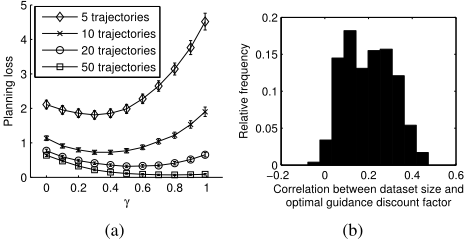
Figure 2a shows the empirical planning loss averaged over datasets as a function of the guidance discount factor γ for a characteristic MDP. Each curve in the figure corresponds to a particular number of trajectories as data. The error bars in this figure and elsewhere show 95% confidence intervals. We can see that the curves exhibit the U-shape predicted by the theory, with minimum planning loss achieved at some γ ⇤ less than γeval. As expected, increasing dataset size reduces planning loss in general, and shifts γ ⇤ to the right.

Figure 2b shows the distribution of the correlation between dataset size and γ ⇤ over 1,000 individual MDPs. This correlation is positive with very high probability, implying that in almost all cases (under RANDOM-MDP) the theoretical relationship between dataset size and γ ⇤ is borne out in practice.

5 Related work

The loss induced by a finite planning horizon is known as truncation loss (see related bounds given by [Kearns et al., 2002]). Separately, it is also well-understood how planning loss relates to model inaccuracy, which can come from estimation error when the model is constructed from data [Mannor et al., 2007; Farahmand et al., 2010], and/or approximation error when approximations are employed in planning (e.g., state abstractions [Ravindran and Barto, 2004]). [Petrik and Scherrer, 2009] showed how a short horizon can reduce loss when the model is inaccurate due to approximation errors. Our work is the first to explore a similar phenomenon due to statistical estimation errors, and our analysis exploits the structure of these errors as well as established principles in supervised learning to obtain stronger claims about γ ⇤ and dataset size.

6 Conclusion

We demonstrated a connection between model complexity and planning horizon by developing a theoretical and empirical analogy to overfitting in supervised learning. We showed that the planning horizon controls the complexity of the policy space, and proved a bound on the loss of the certaintyequivalence policy using a monotonic counting complexity measure. The bound sets up a tradeoff between a term in which a larger planning horizon reduces the loss incurred by certainty-equivalent planning in an accurate model and a term in which a smaller planning horizon reduces the complexity of the policy space and thereby controls overfitting. Empirical results confirm that the optimal choice of guidance discount factor is usually smaller than the discount factor defined by the problem, and that the optimal guidance discount factor increases with the amount of data.

In the longer version of this paper, we also provide another loss bound based on a Rademacher complexity measure, which sets up a similar tradeoff to the one presented here but affords a more general analysis as it removes the assumption in Theorem 2 that the reward function has to be known.

Acknowledgement

This work was supported by NSF grant IIS 1319365. Any opinions, findings, conclusions, or recommendations expressed here are those of the authors and do not necessarily reflect the views of the sponsors.