Online Bellman Residual and Temporal Difference Algorithms with Predictive Error Guarantees

1 Introduction

Reinforcement learning (RL) is an online paradigm for optimal sequential decision making where a agent interacts with environments, takes actions, receives reward and tries to maximize its long-term reward, a discounted sum of all the rewards that will be received from now on. An important part of RL is policy evaluation, the problem of evaluating the expected long-term rewards of a fixed policy. Temporal Difference (TD) learning [Sutton, 1988] is perhaps the best known family of algorithms for policy evaluation. It has been observed that when combined with function approximation, TD may diverge and lead to poor prediction. The Residual Gradient (RG) was proposed [Baird, 1995] to address these concerns. RG attempts to minimize the Bellman Error (BE) (see definition in Sec. 2), typically with linear function approximation, using stochastic gradient descent. Comparison between the family of TD algorithms and RG has received tremendous attention, although most of the analyses heavily rely on certain stochastic assumptions of the environment such as that the sequence of observations are Markovian or from a static Markov Decision Process (MDP). For instance [Schoknecht and Merke, 2003] showed that TD converges provably faster than RG if the value functions are presented by tabular form. [Scherrer, 2010] shows that Bellman Residual minimization enjoys a guaranteed performance while TD does not in general when states are sampled from arbitrary distributions (off-policy) that may not correspond to trajectories taken by the system.

[Schapire and Warmuth, 1996] and [Li, 2008] provided worst-case analysis of long-term predictive error for variants of the linear TD and RG under a non-probabilistic online learning setting. Their results rely on the spectral analysis of a matrix that is related to specific update rules of the TD and RG algorithms under linear function approximation. Unfortunately, this approach makes it more difficult to extend their worst-case (assumption free) analysis to broader families of algorithms and representations that target Bellman and Temporal Difference errors.

Following [Schapire and Warmuth, 1996] and [Li, 2008]'s online learning framework, we present two simple, general connections between long-term predictive error and no-regret online learning that attempts to minimize BE and TD. The central idea is that methods such as TD and RG should be fundamentally understood as online algorithms as opposed to standard gradient methods, and that one cannot simultaneously make consistent predictions in the sense of TD and BE while doing a poor job in terms of long-run predictions. Similar to [Schapire and Warmuth, 1996] and [Li, 2008], our analysis does not rely on any statistical assumptions about the underlying system. This allows us to analyze difficult scenarios such as MDP with transition probabilities changing over time or even with each transition chosen entirely adversarial.

The main contribution of the paper is the analysis of the connections between online long-term reward prediction and no-regret online learning. Particularly, the first analysis on BE shows that any no-regret and stable [Ross and Bagnell, 2011] online learning algorithms, when targeting optimizing BE, ensure small prediction error. The second analysis focuses on TD and shows that when applying the family of Online Mirror Descent (OMD) on TD, we can also achieve small prediction error. We additionally show that Implicit Online Learning is another proper algorithm that can be used for optimizing TD to achieve small prediction error. These two analysis consequently suggests a broad new family of algorithms.

Particularly, our analysis on BE generalizes the RG algorithm from [Baird, 1995] in a sense that RG is a specific example of our family of algorithms that runs Online Gradient Descent (OGD) [Zinkevich, 2003] on a sequence of BE loss functions. For TD, our analysis generalizes TD⇤ (0) from [Schapire and Warmuth, 1996] by showing that running OGD-a special form of OMD, reveals the update rule of TD⇤ (0).

2 Preliminaries

We consider the sequential online learning model presented in [Schapire and Warmuth, 1996; Li, 2008] where no statistical assumptions about the sequence of observations are made. The sequence of the observations can either be Markovian as typically assumed in RL problem settings or even adversarial. We define the observation at time step t as xt 2 Rn , which usually represents the features of the environment at t. Throughout the paper, we assume that feature vector x is bounded as kxk2  X. The corresponding reward at step t is defined as rt 2 R, where we assume that reward is always bounded ♣r♣  R 2 R+. Given a sequence of observations ¶xt♦ and a sequence of rewards ¶rt♦, the long-term reward at t is defined as yt = P1k=t γ k-t rk, where γ 2 [0↪ 1) is a discounted factor. Given a function space F the learner chooses a predictor f at each time step from F for predicting long-term rewards. Throughout this paper, we assume that any prediction made by a predictor f at a state x is upper bounded as ♣f(x)♣  P 2 R+, for any f 2 F and x.

At time step t = 0, the learner receives x0, initializes a predictor f0 2 F and makes prediction ˆ y0 of y0 as f0(x0). Rounds of learning then proceeds as follows: the learner makes a prediction ˆ yt of yt at step t as ft(xt); the learner then observes a reward rt and the next state xt+1; the learner updates its predictor to ft+1. This interaction repeats and is terminated after T steps. Throughout this paper, we call this problem setting as online prediction of long-term reward.

We first define the signed Bellman Error at step t for predictor ft as bt = ft(xt) - rt - γft(xt+1), which measures effectively how self consistent ft is in its predictions between time step t and t + 1. We define the corresponding Bellman Loss at time step t with respect to predictor f as:

We also define signed Temporal Difference Error (signed TD error) at step t for predictor ft as dt = ft(xt) - rt - γft+1(xt+1). We define TD⇤ Loss at step t as:

The Signed Prediction Error of long-term reward at t for ft is defined as et = ft(xt) - yt and e⇤t = f ⇤ (xt) - yt for f ⇤ accordingly. We will typically be interested in bounding the Prediction Error (PE) e2t of a given algorithm in terms of the best possible PE. To lighten notation in the following sections, all sums over time indices implicitly run from 0 to T - 1 unless explicitly noted otherwise.

3 Online Learning for Long-TermReward Prediction

In this section, we first propose a new perspective of RG algorithm and TD⇤ algorithm: we show that RG and TD⇤ both could be understood as running Online Gradient Descent on Bellman loss `bt and TD⇤ loss `dt , respectively.

At every time step t, after receiving the Bellman loss `bt (f), let us apply OGD on `bt (f):

where we denote rff(x) as the functional gradient of the evaluation functional f(x) at function f. 1

Now for linear function approximation where f(x) is represented as wT x, the update step in Eq. 3 exactly reveals the RG algorithm proposed by [Baird, 1995].

Now, let us apply OGD to the TD⇤ loss `dt (f), we get the following update step:

Note that the above update rule is implicit in a sense that the Right Hand Side (RHS) and the Left Hand Side (LHS) both have ft+1 (dt has ft+1). To get the explicit update rule for ft+1, one needs to solve ft+1 from Eq. 4. If we substitute the linear function approximation f(x) = wT x into Eq. 4 and solve for wt+1, one can exactly reveal the TD⇤ (0) update rule proposed in [Schapire and Warmuth, 1996]. 2

Online Gradient Descent is one of the popular no-regret online learning algorithms. The above perspective suggests that RG and TD could be understood as applying a special no-regret online algorithm-OGD, to Bellman loss and TD⇤ loss. A natural question that one would like to know is that whether any other no-regret online algorithms, such as Online Newton step [Hazan et al., 2006], Online Frank Wolf [Hazan and Kale, 2012] and implicit online learning [Kulis et al., 2010], can be applied to Bellman loss `bt and TD⇤ loss `dt , and achieve similar guarantees on PE.

3.1 Optimizing Bellman Loss

In this section, we establish a connection between optimizing Bellman loss and worst case long-term predictive error. Particularly, we show that optimizing Bellman loss with any stable and no-regret online algorithms ensures small prediction error for long-term reward prediction.

We first define the stability condition:

Definition 3.1 Online Stability: For the generated sequence of predictors ft, we say the algorithm is online stable if:

Intuitively, the online stability means that on average the difference between successive predictors is eventually small. That is, the difference between ft(xt+1) and ft+1(xt+1) is small on average. Online stability is a general condition and does not severely limit the scope of the online learning algorithms. For instance, when f is linear, the definition of stability of online learning in [Saha et al., 2012] (see Eq. 3

1 We assume the function rff(x) belongs to F. This is true for function classes such as Reproducing Kernel Hilbert Space (RKHS).

2 This is why we call `dt (f) TD⇤ loss, since with OGD, it reveals the TD⇤ (0) algorithm, not the TD algorithm. However, nearly identical results can be established for TD loss which replaces ft+1 by ft in `dt , and classic TD can be recovered by OGD on TD loss.

in [Saha et al., 2012]) and [Ross and Bagnell, 2011] implies our form of online stability. In fact, we can show that many popular no-regret online learning algorithms including OGD, ONS, OWF, implicit online learning, and FTRL satisfy our online stability condition. We refer reader to [Sun and Bagnell, 2015] for the detailed study of the online stability condition for the above mentioned no-regret online algorithms.

Define ✏t = ft(xt+1)-ft+1(xt+1), with the online stability condition, we now ready to state the main theorem:

Theorem 3.2 Assume a sequence of predictors ¶ft♦ is generated by running some online algorithm on the sequence of Bellman loss ¶`bt ♦. For any predictor f ⇤ 2 F, the sum of prediction errors P e2t can be upper bounded as:

By running a no-regret and online stable algorithm, as T ! 1, the average prediction error is then asymptotically upper bounded by a constant factor of the best possible prediction error in the function class:

The proof of the theorem only consists of easy application of telescoping tricks and Cauchy-Schwart inequalities. We refer readers to [Sun and Bagnell, 2015] for the detailed proof of the above theorem. We emphasize that the above analysis is independent of the particular form of function approximation.

When e⇤t = 0↪ 8t, from Theorem. 3.2, it is easy to see that no-regret rate of (1◁T) P(b2t - b⇤2 t ) and the online stability rate of (1◁T) P ✏2t together determine the rate of the convergence of (1◁T) P e2t . When T ! 1 and γ ! 1 (specifically when γ ≥ (1◁p2)), our upper bound analysis in Eq. 7 is asymptotically tighter than the upper bound in [Li, 2008] (Eq. 12) provided for RG. Since a large number of popular noregret online algorithms satisfy the online stability condition, our theorem essentially expends the family of algorithms that can be used to learn predictors of long-term rewards.

We emphasize here that stability of online algorithms is essential for our results- the no-regret property can be shown by counter-example to be insufficient to achieve low predictive error [Sun and Bagnell, 2015].

3.2 Optimizing TD⇤ Loss

The analysis in Sec. 3.1 is general enough such that almost any existing no-regret online learning algorithm can be used for optimizing Bellman loss and ensures small prediction error on long-term rewards. Though we wish such a nice generalization also exists for TD, we could not establish it. Instead we show that a broad family of online learning algorithmsOnline Mirror Descent (OMD), when applied to TD⇤ loss, ensures small prediction error similar in form to [Schapire and Warmuth, 1996]. We also show that implicit online gradient descent, a special form of implicit online learning, can also be used for optimizing TD⇤ loss. The proofs of the theorems presented in this section are in the appendix. 3

Online Mirror Descent for TD⇤ loss

Let us define R(f) as a regularization and assume that R(f) is a both smooth and strongly convex function with respect to f with norm k · k, defined by the inner product associated with F as kfk2 = hf↪ fi. A function R(f) is ↵-smooth and β-strongly convex if and only if:

Without loss of generality, we assume that R(f) is 1-strongly convex (otherwise simply scale it) and ↵-smooth function with respect to f with norm k · k. For instance, when f is linear, kwk2 ◁2 is 1-strongly convex and 1-smooth. When applying OMD on TD⇤ loss, we have the following update rule, which we denote as OMD-TD⇤ :

Note that when we compute ft using Eq. 9, the RHS of Eq. 9 actually implicitly depends on ˆ yt, which is equal to ft(xt) and hence depends on ft. Here, we assume that though ft appears on both sides of Eq. 9, we can still solve for ft from Eq. 9 as TD⇤ (0) does. In practice, whether or not we can solve ft from Eq. 9 could depend on the form of R(f). For instance, when R(f) = kfk2 ◁2 and f belongs to a Reproducing Kernel Hilbert Space (RKHS) (e.g., linear function f(x) = wT x), we can achieve closed-form update of ft. In fact, when f(x) = wT x, R(w) = kwk2 , it is easy to show the update rule from Eq. 9 reveals the TD⇤ (0) algorithm.

The following theorem shows optimizing TD⇤ loss with OMD ensures small long-term prediction error:

Theorem 3.3 With θ = O( 1 pT ) and F being a RKHS, OMD-TD⇤ (Eq. 9 and 10) has the following bound:

For the average prediction error P e2t ◁T , we have:

Implicit Online Learning for TD⇤ Loss

The OMD framework generalizes quite a few popular online algorithms such as Online Gradient Descent, Normalized Exponential Gradient (normalized EG), OGD with lazy projection and p-norm algorithm [Shalev-Shwartz, 2011]. However, OMD is conceptually different from another family of online algorithms-Implicit Online Learning [Kulis et al., 2010]. Implicit online learning algorithms usually are more stable and robust compared to algorithms with explicit update rules.

3 Available at http://www.cs.cmu.edu/⇠wensun

The idea of implicit update has been applied to classic TD [Tamar et al., 2014], where the authors show the algorithm with implicit update is more stable than classic TD in a sense that it is not sensitive to learning step size.

Briefly, given the sequence of loss `t(f), implicit online learning updates f as ft+1 = argminf `t(f)+ 1 θt DR(f↪ ft), where DR(f↪ ft) is the Bregman divergence generated from regularization R. For special case where f is in RKHS, TD⇤ loss `dt (f) is actually a quadratic loss with respect to f. Hence, we propose to apply the implicit Online Gradient Descent-one special form of implicit online learning, to TD⇤ loss. Set R(f) = kfk2 ◁2, we have the following update rule:

Note that the above update rule is implicit since ˆ yt+1 (buried in `dt ) depends ft+1. Depending on the form of f, we can achieve closed-form solution for ft+1 from Eq. 13.

Below, we demonstrate a closed-form update rule for linear function f(x) = wT x with R(w) = kwk2 . Replace f with w in Eq. 13, take the derivative with respect to w, set it to zero, and solve for wt+1, we will get:

Note that ˆ yt+1 implicitly depends on wt+1. To solve for wt+1, we first dot product xt+1 on both sides of the above equation (the LHS becomes ˆ yt+1), solve for ˆ yt+1 and then substitute ˆ yt+1 back to the equation and solve for wt+1. This gives us the following Implicit-TD⇤ update step:

where bt = (wT t xt - rt - γwT t xt+1). The corresponding update rule for RKHS with kernel K(·↪ ·) is:

where bt = (ft(xt) - rt - γft(xt+1)).

Implicit-TD⇤ has the following upper bound on PE:

Theorem 3.4 With θ = O( 1 pT ) and F being a RKHS, Implicit-TD⇤ (Eq. 15 and 16) has the following bound:

For the average prediction error P e2t ◁T , we have:

3.3 Discussion

The bound of OMD-TD⇤ is the tightest compared to ImplicitTD⇤ and RG. Though our OMD-TD⇤ bound is not as tight as the one from [Schapire and Warmuth, 1996], our analysis is more general. Our bound of RG is asymptotically tighter than the one from [Li, 2008] when γ ! 1. Experimentally we find that Implicit-TD⇤ performs really well, which indicates that our worst-case bound for Implicit-TD⇤ may be not tight.

4 Experiments

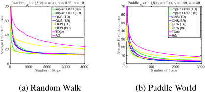
We applied several online learning algorithms to two simulated policy evaluation problems: (1) Random Walk with a ring chain, which is a variant of the Hall problem introduced in [Baird, 1995], (2) PuddleWorld adopted from [Sutton and Barto, 1998]. We tested several popular no-regret and stable online learning algorithms, including implicit online gradient descent (implicit OGD), online Newton step (ONS) [Hazan et al., 2006], online Frank Wolf (OFW) [Hazan and Kale, 2012] and classic online gradient descent [Zinkevich, 2003], on both TD⇤ loss and Bellman loss.

Fig. 1 shows the convergence of average prediction error with respect to number of time steps. We note that ONS and implicit OGD give good convergence speed in general. Throughout the experiments, we found that implicit OGD works well for both TD⇤ loss and Bellman loss. Our experimental results also show that our approaches have the possibility to achieve smaller prediction error than TD(0) (e.g., Fig. 1b). Note that when optimizing TD⇤ loss, ONS and OFW actually achieve good performance, though our analysis on TD⇤ loss currently does not support ONS or OFW.

The experiment results for RKHS can be found at [Sun and Bagnell, 2015], where we also demonstrated these algorithms on a simulated helicopter hover domain [Coates et al., 2008].

5 Conclusion

We introduced a new perspective for RG and TD-they could be understood as running special no-regret online algorithm on Bellman loss and TD⇤ loss, respectively. This new perspective enables us to derive two generalizations, one for RG and one for TD⇤ in the online setting, where no statistical assumptions are placed on the observations. Particularly, we show that any no-regret and stable online algorithms, when applied to Bellman loss, ensures small prediction error. For TD, we connect TD⇤ to two family of online algorithmsOnline Mirror Descent and Implicit Online Learning, and we show that optimizing TD⇤ loss with OMD and implicit OGD guarantees small prediction error. The remaining open problem is that whether there exists a more general connection between TD⇤ loss and no-regret online algorithms: when optimizing TD⇤ loss, are the no-regret property and stability sufficient to achieve low prediction error?