
Inverse Covariance Estimation with Structured Groups
Proceedings of the Twenty-Sixth International Joint Conference on Artificial Intelligence. Main track. Pages 2836-2842.
https://doi.org/10.24963/ijcai.2017/395
Keywords
- Machine Learning: Structured Learning
- Machine Learning: Learning Graphical Models
- Machine Learning: Machine Learning
Abstract
Estimating the inverse covariance matrix of p variables from n observations is challenging when n is much less than p, since the sample covariance matrix is singular and cannot be inverted. A popular solution is to optimize for the L1 penalized estimator; however, this does not incorporate structure domain knowledge and can be expensive to optimize. We consider finding inverse covariance matrices with group structure, defined as potentially overlapping principal submatrices, determined from domain knowledge (e.g. categories or graph cliques). We propose a new estimator for this problem setting that can be derived efficiently via the conditional gradient method, leveraging chordal decomposition theory for scalability. Simulation results show significant improvement in sample complexity when the correct group structure is known. We also apply these estimators to 14,910 stock closing prices, with noticeable improvement when group sparsity is exploited.
- [Agler et al., 1988] Jim Agler, William Helton, Scott McCul- lough, and Leiba Rodman. Positive semidefinite matrices with a given sparsity pattern. Linear algebra and its appli- cations, 107:101-149, 1988.
- [Andersen et al., 2013] Martin S. Andersen, Joachim Dahl, and Lieven Vandenberghe. Logarithmic barriers for sparse matrix cones. Optimization Methods and Software, 28(3):396-423, 2013.
- [Banerjee et al., 2006] Onureena Banerjee, Laurent El Ghaoui, Alexandre d'Aspremont, and Georges Natsoulis. Convex optimization techniques for fitting sparse gaussian graphical models. In Proc. of the 23rd ICML, pages 89-96. ACM, 2006.
- [Banerjee et al., 2008] Onureena Banerjee, Laurent El Ghaoui, and Alexandre d'Aspremont. Model selection through sparse maximum likelihood estimation for multi- variate Gaussian or binary data. JMLR, 9(Mar):485-516, 2008.
- [Chandrasekaran et al., 2012] Venkat Chandrasekaran, Ben- jamin Recht, Pablo A. Parrilo, and Alan S. Willsky. The convex geometry of linear inverse problems. Foundations of Computational mathematics, 12(6):805-849, 2012.
- [Combettes and Pesquet, 2011] Patrick L. Combettes and Jean-Christophe Pesquet. Proximal splitting methods in sig- nal processing. In Fixed-point algorithms for inverse prob- lems in science and engineering, pages 185-212. Springer, 2011.
- [Dahl et al., 2008] Joachim Dahl, Lieven Vandenberghe, and Vwani Roychowdhury. Covariance selection for nonchordal graphs via chordal embedding. Optimization Methods & Software, 23(4):501-520, 2008.
- ['Aspremont et al., 2008] Alexandre d'Aspremont, Onureena Banerjee, and Laurent El Ghaoui. First- order methods for sparse covariance selection. SIAM Journal on Matrix Analysis and Applications, 30(1):56-66, 2008.
- [DeMiguel et al., 2009] Victor DeMiguel, Lorenzo Garlappi, and Raman Uppal. Optimal versus naive diversification: How inefficient is the 1/n portfolio strategy? Review of Financial Studies, 22(5):1915-1953, 2009.
- [Dunn and Harshbarger, 1978] Joseph C Dunn and S Harsh- barger. Conditional gradient algorithms with open loop step size rules. Journal of Mathematical Analysis and Ap- plications, 62(2):432-444, 1978.
- [Frank and Wolfe, 1956] Marguerite Frank and Philip Wolfe. An algorithm for quadratic programming. Naval research logistics quarterly, 3(1-2):95-110, 1956.
- [Friedman et al., 2008] Jerome Friedman, Trevor Hastie, and Robert Tibshirani. Sparse inverse covariance estimation with the graphical LASSO. Biostatistics, 9(3):432-441, 2008.
- [Griewank and Toint, 1984] Andreas Griewank and Philippe L Toint. On the existence of convex decompo- sitions of partially separable functions. Mathematical Programming, 28(1):25-49, 1984.
- [Grone et al., 1984] Robert Grone, Charles R. Johnson, Ed- uardo M. Sá, and Henry Wolkowicz. Positive definite com- pletions of partial hermitian matrices. Linear algebra and its applications, 58:109-124, 1984.
- [Hosseini and Lee, 2016] Mohammad Javad Hosseini and Su- In Lee. Learning sparse gaussian graphical models with overlapping blocks. In Advances in Neural Information Processing Systems, pages 3801-3809, 2016.
- [Hsieh et al., 2013] Cho-Jui Hsieh, Mátyás A Sustik, Inder- jit S Dhillon, Pradeep K Ravikumar, and Russell Poldrack. BIG & QUIC: Sparse inverse covariance estimation for a million variables. In Advances in Neural Information Processing Systems, pages 3165-3173, 2013.
- [Jaggi, 2013] Martin Jaggi. Revisiting Frank-Wolfe: Projection-free sparse convex optimization. In ICML (1), pages 427-435, 2013.
- [Lions and Mercier, 1979] Pierre-Louis Lions and Bertrand Mercier. Splitting algorithms for the sum of two nonlinear operators. SIAM Journal on Numerical Analysis, 16(6):964- 979, 1979.
- [Liu, 1992] Joseph W.H. Liu. The multifrontal method for sparse matrix solution: Theory and practice. SIAM review, 34(1):82-109, 1992.
- [Markowitz, 1952] Harry Markowitz. Portfolio selection. The journal of finance, 7(1):77-91, 1952.
- [Mazumder and Hastie, 2012] Rahul Mazumder and Trevor Hastie. Exact covariance thresholding into connected components for large-scale graphical lasso. JMLR, 13(Mar):781-794, 2012.
- [Meinshausen and Bühlmann, 2006] Nicolai Meinshausen and Peter Bühlmann. High-dimensional graphs and variable selection with the LASSO. The annals of statistics, pages 1436-1462, 2006.
- [Moreau, 1962] Jean-Jacques Moreau. Fonctions convexes duales et points proximaux dans un espace hilbertien. CR Acad. Sci. Paris Sér. A Math, 255:2897-2899, 1962.
- [Negahban et al., 2009] Sahand Negahban, Bin Yu, Martin J. Wainwright, and Pradeep K. Ravikumar. A unified frame- work for high-dimensional analysis of m-estimators with decomposable regularizers. In Advances in Neural Infor- mation Processing Systems, pages 1348-1356, 2009.
- [Obozinski et al., 2011] Guillaume Obozinski, Laurent Ja- cob, and Jean-Philippe Vert. Group LASSO with over- laps: the latent group LASSO approach. arXiv preprint arXiv:1110.0413, 2011.
- [Rolfs et al., 2012] Benjamin Rolfs, Bala Rajaratnam, Do- minique Guillot, Ian Wong, and Arian Maleki. Iterative thresholding algorithm for sparse inverse covariance esti- mation. In Advances in Neural Information Processing Systems, pages 1574-1582, 2012.
- [Scheinberg and Rish, 2009] Katya Scheinberg and Irina Rish. Sinco-a greedy coordinate ascent method for sparse inverse covariance selection problem. preprint, 2009.
- [Yuan and Lin, 2007] Ming Yuan and Yi Lin. Model se- lection and estimation in the Gaussian graphical model. Biometrika, 94(1):19-35, 2007.
- [Yuan, 2012] Xiaoming Yuan. Alternating direction method for covariance selection models. Journal of Scientific Com- puting, 51(2):261-273, 2012.
References were extracted automatically from the PDF and may contain errors.
Full text extracted automatically from the PDF; figures, tables and equations may differ. The PDF is the version of record.
1 Introduction
The inverse covariance matrix is of interest to statisticians in biology, finance, machine learning, etc. In finance, it is a key ingredient for computing value-at-risk, a factor in portfolio optimization. In graphical models, for p random variables with true covariance matrix C, the sparsity pattern of C -1 gives the conditional independence between each pair of variables. However, if n ≪ p, then the sample covariance matrix ˆ C is not invertible, and the pseudoinverse ˆ C † is inaccurately dense. The most popular alternative is the graphical LASSO (G-LASSO) estimator [Yuan and Lin, 2007; Banerjee et al., 2008], the solution to
for some regularization parameter ρ > 0. By adding a sparsityinducing regularizer, the effective degrees of freedom are reduced, and it has been shown that the resulting estimator has a much lower sample complexity than inverting ˆ C. However, this estimator does not incorporate any prior structural knowledge from the problem domain. Additionally, in general solving (1) is computationally challenging if p is large.
Most existing methods for solving (1) require a sequence of eigenvalue decompositions (EDs) [Banerjee et al., 2006; Friedman et al., 2008; d'Aspremont et al., 2008; Yuan, 2012; Rolfs et al., 2012]. This is expensive if p is large; a dense ED requires O(p3 ) computations, and sparse EDs (like Lanczos type methods) are not suitable when the full eigenvalue spectrum is needed. (Used this way, they may be far slower than dense methods.) There are some exceptions; for example [Scheinberg and Rish, 2009] updates each row in a block coordinate descent fashion, and maintains inverses using only rank-2 updates; [Dahl et al., 2008] uses chordal decomposition to compute Newton steps efficiently in an interior point solver; and [Meinshausen and Bühlmann, 2006] uses neighborhood selection, which enforces the conditional independence condition one variable at a time. These methods are more or less intuitive, relying on general convex optimization principles; however, their scalability is limited. On the other end of the spectrum is BIG-QUIC [Hsieh et al., 2013] which can solve up to 1 million variables. This breakthrough method simultaneously makes estimates of the matrix sparsity while also optimizing for it, and updating via block coordinate descent with carefully chosen (non-principal) submatrices. However, it demonstrates the tradeoff between simplicity and scalability; there are many intricate details for a successful implementation.
At the same time, there has been growing interest in the statistics community to exploit group structure in the estimators [Negahban et al., 2009; Chandrasekaran et al., 2012; Obozinski et al., 2011]. For example, [Mazumder and Hastie, 2012] proposes thresholding the sample covariance matrix in order to identify fully-connected components of the graphical model, effectively decomposing (1). More recently, [Hosseini and Lee, 2016] learns overlapping submatrix groups probablistically and penalizes accordingly. To our knowledge, this is the only work that addresses overlapping group sparsity in matrices; however, repeated full EDs are still needed to find the inverse covariance estimate.
We propose an estimator that exploits group structure, where a matrix group is described as either a principal submatrix or the matrix diagonal in Section 2. The solution X is then described as a sum of these possibly overlapping components. We then apply the Frank-Wolfe method to derive the estimator in Section 3. The algorithm at each iteration decomposes into parallelizable eigenvalue computations on the submatrices. In this way, unlike [Mazumder and Hastie, 2012; Hosseini and Lee, 2016], this estimator explicitly uses the predetermined groups as components for decomposition, thus using group structure to improve both performance and computation cost. In Section 4 we give simulation results, which demonstrate that knowing and exploiting group structure significantly improves sample complexity. Finally, in Section 5, we show the performance of our model on the stock datasets.
2 Group NormConstrained Estimator
For an index set γ ⊂ {1, . . . , p} and a vector x ∈ Rp , define xγ as the subvector of x indexed by γ; for the reverse, define the augmenting linear map γ : R|γ| → Rp such that
In [Obozinski et al., 2011], the overlapping group norm is defined as the solution to
for some proper norm ‖·‖ and nonnegative weights w1, . . . , wl. (A common choice is wk = |γk|-1 .) Used as a penalty term or in a constraint, this norm is shown to promote group structure; a small subset of index sets γk are "active", and xi = 0 whenever i is not in an active set.
We extend this concept to matrices, by defining groups implicitly through index sets β ⊂ {1, . . . , p}, where Xβ,β is the submatrix of X selected by the rows and columns indicated by β. Let Sp denote the set of p × p matrices. We define Aβ : S|β| → Sp such that
and extend the overlapping group norm as the solution
Here, X can be considered as the sum of smaller principal submatrices Uk and a diagonal term v, and wk are nonnegative scalar weights. Note that the affine constraint imposes a sparsity pattern on X; if X does not adhere to this pattern (e.g. Xij ̸= 0 for i, j ̸∈ βk, ∀k) then we define ‖X‖G = ∞.
2.1 Our estimator
Given p random variables, define C ∈ Sp and ˆ C ∈ Sp as the true and sample covariance matrices. The group norm regularized graphical LASSO estimator (NG-LASSO) is the solution to
We note that the first two constraints in (4) can be equivalently written as ‖X‖G ≤ α with G-norm defined in (3). As defined, this constraint restricts X to be implicitly within the sparsity pattern defined by the groups βk.
Problem (4) is a computationally tractable approximation of
a natural group norm penalized version of the G-LASSO problem. Specifically, in (5), ‖X‖G can be written in terms of smaller matrices Wk ∈ S|βk| and z ∈ Rp . If additionally the sparsity pattern is chordal (i.e. if the intersection graph of the groups βk is a tree) then the positive semidefinite (PSD) matrix constraint X ⪰ 0 can be decomposed to several smaller matrix constraints, via the equivalence in the following theorem.
Theorem 2.1 [Agler et al., 1988; Griewank and Toint, 1984] ([Grone et al., 1984] dual) If X ∈ Sp has chordal sparsity, corresponding to groups β1, . . . , βl, then
In this case X ⪰ 0 can be decomposed into smaller matrices Uk ∈ S|βk| + and a positive diagonal v ∈ Rp+ (where Sp+ and Rp+ are the PSD cone and nonnegative orthant, both of order p). Then (4) is equivalent to (5) if and only if at optimality, Wk = Uk for all k, and v = z.
3 Optimization
The Frank-Wolfe algorithm has regained much attention in minimizing sparse problems [Jaggi, 2013], mimicking greedy approaches yet having guaranteed optimality for convex problems. The Frank-Wolfe algorithm for solving minX{f(X) : X ∈ D} is described in Alg. 1. Using step sizes η[t] =
Algorithm 1 One step of Frank-Wolfe algorithm
Input: X[t] ∈ D, t-th iteration, step size η
- 1: Compute gradient ∇f(X[t] )
- 2: Compute forward step : S = argminS∈D〈U,∇f(X[t] )〉
- 3: Update primal variable : X[t+1] = (1 - η[t] )X[t] + η[t]S Output: optimal X[t+1]
2/(t + 2), it is known that the iterates of algorithm 1 converge at the sublinear rate of O(1/t) [Frank and Wolfe, 1956; Dunn and Harshbarger, 1978]. We apply this algorithm for problem (4).
Forward step At each iteration, the forward step consists of l parallelizable projections on cones C1, . . . , Cl. Specifically, at each forward step, we compute
where index j = argmaxk w-1 k ‖Zk‖F and Zj = projCj (-∇f (X)βj ,βj ). Then S = ∑k wkAβk,βk (Uk). The derivations are given in appendix A.
Gradient computation In general, to compute the gradient ∇(log det(X)) = X-1 requires matrix inversion, which negates the computational complexity gain by decomposing the PSD cone. However, if the groups βk form a chordal pattern, fast inversion methods exist [Liu, 1992; Andersen et al., 2013] which require at each step l inversions of matrices at most of order |βk|.
Applying both techniques, Alg. 2 describes the procedure for one iteration to find the NG-LASSO estimator (4). The
Algorithm 2 One step of Frank-Wolfe algorithm for (4)
Input: X[t] ∈ D, t-th iteration, step size η := 2 t+2
- 1: Find ∇f(X) =X-1 +C
- 2: Find the forward direction U +:
- 3: Update X[t+1] =X[t] + 2 t+2 U +
Output: X[t+1] .
main computational bottleneck at each step is a sequence of EDs of the submatrices ∇f(X)βk,βk , both for inverting X and for projecting on the PSD cone. For both operations, the complexity is O(|βk|3 ) per group. If |βk| < p/l excluding the diagonal group, then the total per-iteration complexity of the proposed optimization procedure has a per-iteration complexity of O(p3 /l2 + p), and much smaller than O(p3 ) for G-LASSO.
4 Numerical Simulations
Here we show two simulation results: one on a general group sparsity pattern, and the other on a specific chordal pattern (banded).
To pick α and ρ, we swept powers of two in {2-5 , . . . , 25 } and picked the best performing ρ or α for each test. In cases where the best performing ρ or α was on the boundary, additional parameters were tested until this was no longer the case.
4.1 Baselines
As one baseline, we solve (1). However, since group structure also reveals matrix sparsity, for fair comparison we also solve
(1) restricted to the sparsity pattern induced by the groups:
which we call restricted group LASSO (RG-LASSO). We solve these baselines using the Douglas-Rachford method [Lions and Mercier, 1979; Combettes and Pesquet, 2011] for minimizing the sum of m convex functions, 1 detailed exactly as in [Combettes and Pesquet, 2011], Alg 10.27, with
and f3, f4 as indicator functions for constraints
The proximal operator [Moreau, 1962] for a convex function f(X) is defined as
and is defined for all Z, even if Z is not in the domain of f. (This is especially useful for f = log det and Z ̸⪰ 0.) From optimality conditions, it can be shown that
where V diag(d)V T is the eigenvalue decomposition of t ˆ C-Z. Similarly, proxtf2 is the well-known shrinkage operator, and proxtf3 , proxtf4 are projections on their respective constraint spaces.
4.2 Random sparsity
For X ∈ Sp , we randomly select l groups βk ⊂ {1, . . . p} of size b, and assume that this is the known group structure. Additionally, we select ⌈σG · l⌉ "active" groups (for 0 < σG < 1); the identity of these groups are not known in training. In this simulation, we investigate the sample size required to recover the active groups, comparing G-LASSO, RG-LASSO, and NG-LASSO. In general, the sparsity patterns here are not chordal.
To determine the sparsity pattern of X, i.e.the estimate of C -1 , we threshold so that
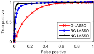
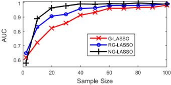
for θ ∈ [0, 1]. Figure 1 shows the receiver operating characteristic (ROC) curve for p = 100 variables and n = 25 samples, where θ is implicitly swept. It is clear that NG-LASSO outperforms both other estimators; however, it is also evident that restricting the sparsity already offers much improvement. In order to remain agnostic to the right choice of θ, we use the area under the ROC curve (AUC) as the primary metric of estimator quality. Figure 2 plots the AUC for varying sample sizes n. Again, it is clear that for most cases, NG-LASSO outperforms RG-LASSO and G-LASSO. The exception is at very small values of n, where the number of observations is too low.
1 This ADMM-type of method has the advantage over the projected gradient method because it has no step size restrictions based on the objective function's Lipschitz constant, which for log det is unbounded.
4.3 Banded sparsity
Next, we present a more extensive experiment with a chordal sparsity pattern; specifically, a banded pattern. For X ∈ Sp , we assume that the true sparsity pattern consists of a nonzero diagonal and some active diagonal blocks of size b, where b is known but the true sparsity pattern is not. This gives in total l = p - b + 1 candidate groups βk = {k, · · · , k + b} for k = 1, · · · , l. Among l groups, we assume σGl groups are active (where 0 < σG < 1). Moreover, we simulate in-group sparsity; that is, for 0 < σI ≤ 1, we fix Pr(Xij ̸= 0|i, j ∈ βk) = σI . Note that using only known information, we must assume the sparsity pattern is banded with bandwidth b.
We construct an invertible C -1 with the true sparsity pattern, and form a sample covariance matrix ˆ C by sampling from a multivariate Gaussian with 0 mean and covariance C. The goal is to use the estimators to correctly recover the sparsity pattern of C using ˆ C where the number of observations n is as small as possible.
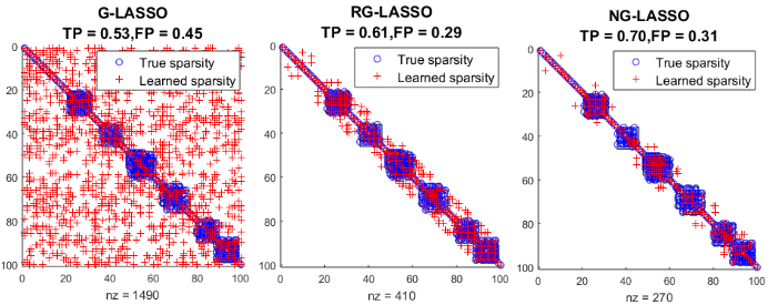
Figure 3 shows a small example when p = 100, n = 50 and σI = 0.25. There are in total 90 groups in the banded sparsity pattern, where the 9 active groups (true sparsity) are in blue. We pick the estimator nonzeros by thresholding on the absolute value, choosing the threshold to, in each case, maximize min{# true positives, # true negatives}.
It is clear that, for this small example, G-LASSO (left) yields many spurious nonzeros. By simply restricting the sparsity pattern to B, the performance of RG-LASSO (center) already improves significantly, but NG-LASSO is still the best, since it accounts for sparsity in group selection as well.
Table 1 gives the result of a more extensive experiment, where the threshold, α, and ρ are picked to maximize the AUC, which is given for several p, n and σI . Here, we see that NGLASSO is comparable with RG-LASSO when p ≈ n, but is consistently better for p ≫ n; both, however, are considerably improved over G-LASSO.
| p | n | σI | ˆ C | ˆ C† | G | RG | NG |
|---|---|---|---|---|---|---|---|
| 100 | 10 | 0.1 | 0.43 | 0.44 | 0.50 | 0.57 | 0.65 |
| 100 | 10 | 0.25 | 0.39 | 0.40 | 0.48 | 0.58 | 0.64 |
| 100 | 100 | 0.1 | 0.59 | 0.60 | 0.89 | 0.88 | 0.88 |
| 100 | 100 | 0.25 | 0.52 | 0.69 | 0.83 | 0.80 | 0.85 |
| 1000 | 10 | 0.1 | 0.41 | 0.41 | 0.49 | 0.52 | 0.63 |
| 1000 | 10 | 0.25 | 0.34 | 0.34 | 0.40 | 0.38 | 0.68 |
| 1000 | 100 | 0.1 | 0.55 | 0.56 | 0.56 | 0.58 | 0.89 |
| 1000 | 100 | 0.25 | 0.48 | 0.49 | 0.48 | 0.52 | 0.90 |
| Per Iteration | Overall | ||||||
|---|---|---|---|---|---|---|---|
| p | n | G | RG | NG | G | RG | NG |
| 100 | 10 | <0.1 | <0.1 | <0.1 | 0.94 | 3.93 | 7.3 |
| 100 | 100 | <0.1 | <0.1 | <0.1 | 0.19 | 0.17 | 0.39 |
| 1000 | 10 | 1.6 | 1.6 | 0.35 | 93.6 | 108.69 | 351.1 |
| 1000 | 100 | 1.4 | 1.4 | 0.35 | 13.8 | 9.97 | 349.5 |
| 2500 | 100 | 21.3 | 19.6 | 1.1 | 852.9 | 556.7 | 333.9 |
| 5000 | 100 | 150.9 | 125.8 | 1.7 | - | - | - |
Table 2 gives the per-iteration and total runtime of the three methods. In all cases, the per-iteration runtime depends only on p and b, and for larger p, NG-LASSO enjoys a much smaller per-iteration runtime. Of course, the total runtime (influenced also by the number of iterations) is also important; however, our experiments suggest this value is much less predictable. Several trends do emerge, though; for all methods, the runtime grows significantly when n is very small or σI is very low, suggesting that problem conditioning influences convergence rate as well. However, the key takeaway is that for very large p it is impossible to maintain full EDs for each iteration, and some decomposition must be used.
5 Financial application
In this section, we examine the performance of G-LASSO, RG-LASSO, and NG-LASSO in estimating the inverse covariance matrix for 14910 stocks, over a period of 100 or fewer days. This problem arises in finance in Markowitz portfolio optimization [Markowitz, 1952], which discusses optimal portfolio allocations using only mean and covariance information. Specifically, when the objective is to minimize return volatility, it is advised to invest in each stock a weight wi of one's assets, where w minimizes the following quadratic optimization problem
with optimal solution w = (1T C -11)-1C -11. However, in practice it is very difficult to apply this principle to large markets, especially when the amount of available historical data is limited, as the exact problem that C -1 is hard to estimate when p (thousands of stocks) is much greater than n (at most a few hundred days' opening or closing prices); using Markowitz' method in this regime can consistently underperformmuch simpler methods [DeMiguel et al., 2009]. Thus, there is great interest in applying sparse estimators for a more generalizable calculation.
We attempt to estimate the inverse covariance matrix for stocks obtained from Yahoo! Finance, using daily closing prices as features. Details on the data scraping are given in appendix B. Define ui as the full length observation vector for stock i, and Si as the set of indices of ui where that stock price observation is available. Define V = {1, 2, . . . , 100}, T = {101, 102, . . . , 200}, and R = {201, 202, . . . , 200 + n} as the indices of a validation, test, and train set respectively, and for all stocks i, Vi = V ∩ Si, Ti = T ∩ Si, Ri = R ∩ Si. 2 The sample covariance is then calculated as
We solve (1), (6), and (4) sweeping ρ, α for powers of 2 from 2-5 to 25 , using cross validation to pick the best ρ and γ. 3
Unlike the controlled simulation, we have no real understanding of the ground truth, so we test the estimator's generalizability, by measuring the maximum likelihood over the test samples. Specifically, we compute the negative log likelihood (NLL) for precision matrix X and samples {ui}i∈T in the test set:
2 Not every day's value is provided for every stock.
3 As before, if the best ρ or α is on the boundary, additional powers of 2 are computed until this is no longer the case.
| sectors | industry | |||||
|---|---|---|---|---|---|---|
| p | n | G | RG | NG | RG | NG |
| 100 | 10 | 2.2e2 | 2.5e2 | 7.0e2 | 2.7e2 | 5.5e2 |
| 500 | 10 | 2.0e3 | 1.8e3 | 3.7e3 | 1.3e3 | 3.5e3 |
| 500 | 100 | 1.3e3 | 9.1e2 | 4.1e3 | 9.3e2 | 3.1e3 |
| 1000 | 10 | 2.5e3 | 2.6e3 | 7.9e3 | 2.8e3 | 6.1e3 |
| 1000 | 100 | 1.1e13 | 4.4e3 | 7.1e3 | 4.4e3 | 7.4e3 |
| 2500 | 100 | - | 1.1e4 | 3.9e4 | 1.1e4 | 1.7e4 |
| 5000 | 100 | - | 1.5e12 | 1.1e7 | 5.9e10 | 7.9e4 |
| 14910 | 100 | - | - | 8.6e12 | - | 5.2e5 |
In this case, the smaller the value, the better.
Table 3 gives the test NLL for various p and n. As p grows (and especially as p/n grows) it is clear that G-LASSO has poorer performance, though the behavior is not as consistent as in table 1. Additionally, it seems that restricting the sparsity pattern gives the regularization needed to achieve very good performance, though we note that for very large p, NG-LASSO still does better.
Table 4 gives the runtime of each experiment for the best set of parameters, showing 1) the time to do one set of EDs (p × p for LASSO and sum of |βk| × |βk|, k = 1, . . . l for group methods), 2) the average per-iteration runtime (≈ 1 ED) and 3) the total runtime. Since in this application all groups are nonoverlapping (all stocks are assigned a single sector and industry) computing RG-LASSO can be done in a fully decomposable manner, and can run at the same periteration speed as NG-LASSO. However, because the DouglasRachford method requires keeping 9 copies of the variables as separate iterates, it runs out of memory at p = 14910. Therefore our method still maintains the scalability advantage.
6 Conclusion
We present an inverse covariance estimator that regularizes for overlapping group sparsity, and provide better estimates when p ≫ n. This is a challenging problem, common in finance, climate research, bioinformatics etc.. The techniques we present here incorporate known group structure in a principled way, and practically such that the group structure itself can be used to incorporate decomposition. A natural extension, and an avenue for future work, is to apply it to applications where group structure is not known, but can be ascertained through unsupervised methods, like K-means, spectral clustering, etc..
| p | 500 | 1000 | 2500 | 5000 | 14910 |
|---|---|---|---|---|---|
| p×p ED | < 0.1 | 3.4e-1 | 5.2 | 4.3e1 | 1.1e3 |
| S-ED | < 0.1 | < 0.1 | 1.4e-1 | 6.4e-1 | 1.5e1 |
| I-ED | < 0.1 | < 0.1 | < 0.1 | < 0.1 | 1.0 |
| G 1 it. | 0.381 | 1.33 | 20.5 | 150.5 | - |
| RG (S) 1 it. | < 0.1 | 0.20 | 1.6 | 6.0 | - |
| RG (I) 1 it. | < 0.1 | 0.17 | 0.74 | 2.3 | - |
| NG (S) 1 it. | < 0.1 | 0.20 | 1.4 | 5.5 | 79.6 |
| NG (I) 1 it. | < 0.1 | 0.18 | 0.72 | 2.2 | 20.2 |
| G all | 20.0 | 1324.2 | - | - | - |
| RG (S) all | 3.0 | 88.9 | 713.6 | 34.7 | - |
| RG (I) all | 2.5 | 74.0 | 341.5 | 2351.1 | - |
| NG (S) all | 2.5 | 29.8 | 169.1 | 560.7 | 80377.2 |
| NG (I) all | 4.6 | 26.9 | 79.7 | 677.2 | 2149.5 |
Acknowledgements
This research was supported in part by NSF grant IIS-1319749.
Appendix
A Forward step derivation
The following is the derivation for Frank-Wolfe forward step in solving (4), which can be applied to more general problems. We first reformulate (4) into a generalized vector optimization problem:
where
Here f(x) can be any differentiable convex function, and C1, . . . , Cl are proper convex cones. The index γ1, . . . , γl define the groups. The vector variables are uk ∈ R|γ| , As before, the parameters w1, . . . , wl > 0 are weights. Problem (4) is a special case of (7). To match βk with the sets γk, the equivalence is such that vec(Aβk,βk ) = vec(A)γk . The forward step to (7) is then
For notational convenience, define ck = vec(∇f(X)γk ) for k = 1, . . . , l. Then we can rewrite the objective function in (9) as
with constraints unchanged. FromMoreau's decomposition, any vector a can be written as the sum of its projection on a closed convex cone C and its polar cone C ◦ , of which are orthogonal. If we then expand
then since feasible uk ∈ Ck, by definition of polar cone projC◦ k (ck)T uk ≤ 0, and = 0 only if uk = skprojCk (ck). This is the optimal choice of direction for uk, since it also maximizes the first term projCk (ck)T uk, and does not affect the norm constraint. If we additionally define scalars
then an even simpler equivalent formulation is
which is a linear program with a known optimal solution of
Substituting gives the closed form solution in the text.
B Yahoo! Finance data scraping details
Using the Yahoo! ticker downloader 4 we downloaded 27684 tickers for different stocks. We then used the Yahoo! finance API 5 to gather daily open, high, low, close, volume, and adjusted closing prices. We chose to monitor daily closing prices. We define groups as industries or sectors, as described in https://biz.yahoo.com/p/.
Any stock that we could not identify with an industry and sector was removed. We then prune the data to make sure it is as dense as possible. This resulted in 14,910 stocks and 1,005 daily closing prices. In total there are 9 sectors and 214 industries. with an average sector size 1656.7 and industry size 69.3. All stock vectors were then demeaned.
@inproceedings{ijcai2017p395,
  title     = {Inverse Covariance Estimation with Structured Groups},
  author    = {Tao, Shaozhe and Sun, Yifan and Boley, Daniel},
  booktitle = {Proceedings of the Twenty-Sixth International Joint Conference on
               Artificial Intelligence, {IJCAI-17}},
  publisher = {International Joint Conferences on Artificial Intelligence Organization},
  editor    = {Carles Sierra},
  pages     = {2836--2842},
  year      = {2017},
  month     = {8},
  note      = {Main track},
  doi       = {10.24963/ijcai.2017/395},
  url       = {https://doi.org/10.24963/ijcai.2017/395},
}
TY - CPAPER TI - Inverse Covariance Estimation with Structured Groups AU - Tao, Shaozhe AU - Sun, Yifan AU - Boley, Daniel T2 - Proceedings of the Twenty-Sixth International Joint Conference on Artificial Intelligence, IJCAI-17 PB - International Joint Conferences on Artificial Intelligence Organization PY - 2017 SP - 2836 EP - 2842 DO - 10.24963/ijcai.2017/395 UR - https://doi.org/10.24963/ijcai.2017/395 ER -Copied
Machine-readable versions of this paper, for tools and AI agents:





