
Joint Image Emotion Classification and Distribution Learning via Deep Convolutional Neural Network
Proceedings of the Twenty-Sixth International Joint Conference on Artificial Intelligence. Main track. Pages 3266-3272.
https://doi.org/10.24963/ijcai.2017/456
Keywords
- Machine Learning: Transfer, Adaptation, Multi-task Learning
- Multidisciplinary Topics and Applications: AI and Ubiquitous Computing Systems
- Machine Learning: Multi-instance/Multi-label/Multi-view learning
Abstract
Visual sentiment analysis is attracting more and more attention with the increasing tendency to express emotions through visual contents. Recent algorithms in convolutional neural networks (CNNs) considerably advance the emotion classification, which aims to distinguish differences among emotional categories and assigns a single dominant label to each image. However, the task is inherently ambiguous since an image usually evokes multiple emotions and its annotation varies from person to person. In this work, we address the problem via label distribution learning (LDL) and develop a multi-task deep framework by jointly optimizing both classification and distribution prediction. While the proposed method prefers to the distribution dataset with annotations of different voters, the majority voting scheme is widely adopted as the ground truth in this area, and few dataset has provided multiple affective labels. Hence, we further exploit two weak forms of prior knowledge, which are expressed as similarity information between labels, to generate emotional distribution for each category. The experiments conducted on both distribution datasets, i.e., Emotion6, Flickr_LDL, Twitter_LDL, and the largest single emotion dataset, i.e., Flickr and Instagram, demonstrate the proposed method outperforms the state-of-the-art approaches.
- [Borth et al., 2013] Damian Borth, Rongrong Ji, Tao Chen, Thomas Breuel, and Shih-Fu Chang. Large-scale visual sentiment ontology and detectors using adjective noun pairs. In MM, 2013.
- [Campos et al., 2015] Víctor Campos, Amaia Salvador, Xavier Giro-i Nieto, and Brendan Jou. Diving deep into sentiment: Understanding fine-tuned cnns for visual sentiment prediction. In ACM ASM, 2015.
- [Chang and Lin, 2011] Chih-Chung Chang and Chih-Jen Lin. Libsvm: a library for support vector machines. TIST, 2(3):27, 2011.
- [Chen et al., 2014] Tao Chen, Damian Borth, Trevor Dar- rell, and Shih-Fu Chang. Deepsentibank: Visual sentiment concept classification with deep convolutional neural net- works. arXiv preprint arXiv:1410.8586, 2014.
- [Deng et al., 2009] Jia Deng, Wei Dong, Richard Socher, Li- Jia Li, Kai Li, and Li Fei-Fei. Imagenet: A large-scale hierarchical image database. In CVPR, 2009.
- [Gao et al., 2017] Bin-Bin Gao, Chao Xing, Chen-Wei Xie, Jianxin Wu, and Xin Geng. Deep label distribution learn- ing with label ambiguity. TIP, 2017.
- [Geng et al., 2013] Xin Geng, Chao Yin, and Zhi-Hua Zhou. Facial age estimation by learning from label distributions. TPAMI, 35(10):2401-2412, 2013.
- [Geng, 2016] Xin Geng. Label distribution learning. TKDE, 28(7):1734-1748, 2016.
- [Jia et al., 2012] Jia Jia, Sen Wu, Xiaohui Wang, Peiyun Hu, Lianhong Cai, and Jie Tang. Can we understand van gogh's mood? learning to infer affects from images in so- cial networks. In ACM MM, 2012.
- [Krizhevsky et al., 2012] Alex Krizhevsky, Ilya Sutskever, and Geoffrey E Hinton. Imagenet classification with deep convolutional neural networks. In NIPS, 2012.
- [Lu et al., 2012] Xin Lu, Poonam Suryanarayan, Reginald B Adams Jr, Jia Li, Michelle G Newman, and James Z Wang. On shape and the computability of emotions. In ACM MM, 2012.
- [Machajdik and Hanbury, 2010] Jana Machajdik and Allan Hanbury. Affective image classification using features in- spired by psychology and art theory. In ACM MM, 2010.
- [Mikels et al., 2005] Joseph A Mikels, Barbara L Fredrick- son, Gregory R Larkin, Casey M Lindberg, Sam J Maglio, and Patricia A Reuter-Lorenz. Emotional category data on images from the international affective picture system. Behavior research methods, 37(4):626-630, 2005.
- [Mirzazadeh et al., 2015] Farzaneh Mirzazadeh, Siamak Ra- vanbakhsh, Nan Ding, and Dale Schuurmans. Embedding inference for structured multilabel prediction. In NIPS, 2015.
- [Nicolaou et al., 2011] Mihalis A Nicolaou, Hatice Gunes, and Maja Pantic. A multi-layer hybrid framework for di- mensional emotion classification. In ACM MM, 2011.
- [Pang and Ngo, 2015] Lei Pang and Chong-Wah Ngo. Mut- limodal learning with deep boltzmann machine for emo- tion prediction in user generated videos. In ICMR, 2015.
- [Peng et al., 2015] Kuan-Chuan Peng, Tsuhan Chen, Amir Sadovnik, and Andrew C Gallagher. A mixed bag of emo- tions: Model, predict, and transfer emotion distributions. In CVPR, 2015.
- [Plutchik, 1980] Robert Plutchik. A general psychoevolu- tionary theory of emotion. Theories of emotion, 1:3-31, 1980.
- [Plutchik, 2001] Robert Plutchik. The nature of emotions. American Scientist, 89(4):344-350, 2001.
- [Rao et al., 2016] Tianrong Rao, Min Xu, and Dong Xu. Learning multi-level deep representations for image emo- tion classification. arXiv preprint arXiv:1611.07145, 2016.
- [Simonyan and Zisserman, 2014] Karen Simonyan and An- drew Zisserman. Very deep convolutional networks for large-scale image recognition. In arXiv preprint arXiv:1409.1556, 2014.
- [Sun et al., 2016] Ming Sun, Jufeng Yang, Kai Wang, and Hui Shen. Discovering affective regions in deep convo- lutional neural networks for visual sentiment prediction. In ICME, 2016.
- [Szegedy et al., 2016] Christian Szegedy, Vincent Van- houcke, Sergey Ioffe, Jon Shlens, and Zbigniew Wojna. Rethinking the inception architecture for computer vision. In CVPR, 2016.
- [Yang et al., 2017] Jufeng Yang, Ming Sun, and Xiaoxiao Sun. Learning visual sentiment distribution via augmented conditional probability neural network. In AAAI, 2017.
- [You et al., 2015] Quanzeng You, Jiebo Luo, Hailin Jin, and Jianchao Yang. Robust image sentiment analysis using progressively trained and domain transferred deep net- works. In AAAI, 2015.
- [You et al., 2016] Quanzeng You, Jiebo Luo, Hailin Jin, and Jianchao Yang. Building a large scale dataset for image emotion recognition: The fine print and the benchmark. In AAAI, 2016.
- [Zhao et al., 2014] Sicheng Zhao, Yue Gao, Xiaolei Jiang, Hongxun Yao, Tat-Seng Chua, and Xiaoshuai Sun. Ex- ploring principles-of-art features for image emotion recog- nition. In ACM MM, 2014.
- [Zhao et al., 2015] Sicheng Zhao, Hongxun Yao, Xiaolei Jiang, and Xiaoshuai Sun. Predicting discrete probability distribution of image emotions. In ICIP, 2015.
- [Zhao et al., 2016] Sicheng Zhao, Hongxun Yao, Yue Gao, Rongrong Ji, Wenlong Xie, Xiaolei Jiang, and Tat-Seng Chua. Predicting personalized emotion perceptions of so- cial images. In MM, 2016.
References were extracted automatically from the PDF and may contain errors.
Full text extracted automatically from the PDF; figures, tables and equations may differ. The PDF is the version of record.
1 Introduction
Understanding the sentiment implied in images has attracted many interests due to its various applications [Jia et al., 2012; Borth et al., 2013]. Inspired by the psychology and principles of art, a lot of work investigate the different groups of manually crafted features [Machajdik and Hanbury, 2010; Zhao et al., 2014], with the goal of automatically assigning a single emotion to each image. In the last few years, with the rapid popularity of CNNs, the researchers [You et al., 2016; Sun et al., 2016] also apply CNNs to recognize image sentiment and illustrate the superior performance of the deep features against the hand-tuned features [Rao et al., 2016].
However, compared to traditional vision tasks, analyzing images at affective level is inherently challenging. The affective image rarely expresses pure emotion, but often a mixture of different emotions [Plutchik, 1980; Zhao et al., 2014]. In addition, people with diverse social and culture background may have different emotional reactions to the same image. Figure 1 shows three samples from the newly published Flickr LDL dataset [Yang et al., 2017], and the annotators do not reach an agreement on any image. As can be seen, there exists label ambiguity among the emotions, which refers to the uncertainty of the "ground-truth label". While most work assign the dominant votes as the groundtruth [Machajdik and Hanbury, 2010; You et al., 2016], such ambiguity characteristic is ignored, making it difficult to learn robust emotional representations for predicting the image labels.
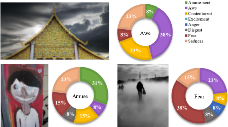
We develop a deep multi-task framework to address the problem, in which the softmax is employed as the classification constraints, and the Kullback-Leibler (KL) loss is added for distribution learning. For the distribution datasets which have the detailed annotations from different users, we explicitly use the votes as the ground truth label distributions in the training phase. During the joint optimization process, the tasks of emotion classification and distribution prediction boost each other with the help of the rich sentiment relations. On the other hand, the majority voting scheme is widely adopted in this area, and most current datasets are single label datasets. We exploit two weak prior knowledge to generate the distributions on these datasets for training. Inspired by [Zhao et al., 2016], pairwise emotion distance can be defined according to Mikels' wheel [Mikels et al., 2005] (see Figure 2), and it is obvious that there exists hierarchical structure among the sentiment labels. For example, Amusement, Contentment, Awe, Excitement are positive emotions, and Sadness, Anger, Fear, Disgust are negative ones. In this work, based on the similarity of the pairwise sentiment, we generate the distributions with the Gaussian function following [Geng et al., 2013]. Different from the previous work which take the label ambiguity into account and aim to predict the probability distribution of the categorical image emotions [Zhao et al., 2015; Peng et al., 2015; Yang et al., 2017], our proposed multi-task framework simultaneously optimizes the classification and the label distribution prediction, performing better on both distribution datasets (Emotion6, Flickr LDL, Twitter LDL), and single label dataset (Flickr and Instagram).
Our contributions are summarized as follows. First, we address the challenges of visual sentiment analysis by a multitask deep learning framework, which can learn the sentiment representations among ambiguous emotional categories in an end-to-end manner. Second, we also extend our method to single label datasets using two strategies to transform the dominant sentiment label into distribution and incorporate label ambiguity into the learning process, with which the classification performance is boosted. We will release the code, models and results for accessible reproducible research.
2 RelatedWork
The general literature on visual sentiment analysis ranges from still images [Machajdik and Hanbury, 2010] to videos [Pang and Ngo, 2015]. In this section, we focus on reviewing the related work on affective image prediction, especially deep learning based methods, and label distribution learning algorithms.
2.1 Image Emotion Classification
Previous work of image emotion classification can be roughly divided into dimensional approaches [Nicolaou et al., 2011; Lu et al., 2012] and categorical approaches [Machajdik and Hanbury, 2010; Zhao et al., 2014]. The dimensional approaches represent sentiment in a two- or three-dimensional space, and the categorical approaches map sentiment into one of the representative categories, which is straightforward for people to understand and thus have been widely applied in recent studies. Most previous work on image emotion analysis use the elements-of-the-art based low-level features. [Machajdik and Hanbury, 2010] defines a combination of rich handcrafted features based on art and psychology theory, including composition, color variance and image semantics. [Zhao et al., 2014] introduces more robust and invariant visual features designed according to art principles. These hand-crafted visual features are proven to be effective on several small datasets, whose images are selected from a few specific domains, e.g. abstract paintings and art photos [Machajdik and Hanbury, 2010].
More recently, considering the success of CNN-based approaches in many computer vision tasks, CNN has also been employed for sentiment representation and achieves significant advance. [Chen et al., 2014] constructs DeepSentiBank as a visual sentiment concept (adjective-noun pairs, ANP) classification model, which are useful as effective statistical cues for detecting emotions depicted in the images. Several work incorporate the model weights learned from a large-scale general dataset [Deng et al., 2009] and finetune the state-of-the-art CNNs for the task of visual emotion prediction [Campos et al., 2015]. [You et al., 2015; 2016] propose a novel progressive CNN architecture, namely PCNN, to make use of large noisy web data, and further perform benchmarking analysis on the Flickr and Instagram (FI) dataset, which is currently the largest single label dataset containing 23,308 affective images. In [Rao et al., 2016], a multi-level deep network (MldeNet) is proposed to unify both low-level and high-level information of images. The existing CNN frameworks on visual sentiment analysis can be viewed as classification [You et al., 2016] and regression [Peng et al., 2015] models, which employ the softmax loss to maximize the probability of the correct class or Euclidean loss to minimize the squares difference between the prediction and the ground truth. However, both of the optimization objective functions fail to utilize sentiment ambiguity and similarity information among image categories.
2.2 Label Distribution Learning
[Geng, 2016] proposes a novel machine learning paradigm for describing the exact role of each label, which contains three strategies for the algorithms, i.e. problem transfer (PT), algorithm adaption (AA), and specialized algorithms (SA). To the best of our knowledge, few work has paid attention to such detailed ambiguity information for visual sentiment analysis. [Zhao et al., 2015] proposes to predict the probability distribution with shared sparse learning model using lowlevel features. [Peng et al., 2015] trains regressions utilizing the deep CNN with the Euclidean loss for each emotion category, whose outputs are then normalized to be the probabilities of each class. Based on a state-of-the-art condition probability neural network (CPNN) [Geng et al., 2013], BCPNN and ACPNN [Yang et al., 2017] are developed for predicting sentiment distribution. However, CPNN-based methods are only designed as a three layer neural network classifier, taking the off-the-shelf features as input. Such methods are suboptimal since the extracted features do not consider the correlation between labels during leaning. More recently, DLDL is proposed to learn the label distribution using the deep neural network for tasks with continuous labels, e.g. age estimation and head pose estimation [Gao et al., 2017]. Since DLDL minimizes a Kullback-Leibler divergence between the predicted and the ground-truth distributions, the dominant label may be confused in predicting.
3 Methodology
For an affective image x, the description degree l = {li}Ci=1 is assigned to each emotion label of C classes representing the degree to which the emotion describes the image, where
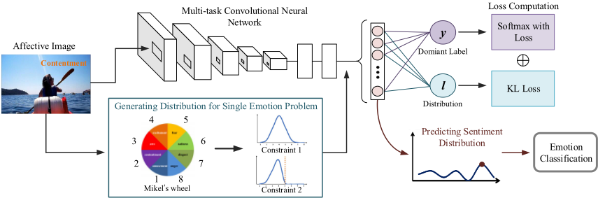
∑Ci=1 li = 1 and li ∈ [0, 1]. For the distribution datasets, we explicitly use the votes as the ground truth label distribution. As illustrated in Figure 2, we employ the proposed deep multi-task framework to simultaneously optimize classification and distribution prediction according to the label distribution l ∈ RC . In addition, we also propose two strategies to convert the single emotion to the distribution for training on the single label datasets.
3.1 Converting Single Emotion Problem
The majority voting scheme is widely adopted to obtain the single emotion ground truth in most datasets [Machajdik and Hanbury, 2010; You et al., 2016]. Since few dataset provides the manually annotated sentiment distribution, we propose to generate l from the single label. Inspired by that there are different similarities between the pairwise emotion categories [Plutchik, 2001], we fix the order of sentiment labels according to Mikels' wheel [Zhao et al., 2016] and thus the distance can be defined by counting the number of steps from one emotion to another. We let li > lj if the distance between the i-th emotion and the ground-truth is smaller than the one between the j-th emotion and the ground-truth.
In terms of logical relationships between labels, there are two common forms in multi-label classification, i.e. implication and exclusion [Mirzazadeh et al., 2015]. For implication, it would like to enforce relationships of the form Yi ⇒ Yj, which means that whenever the label Yi is set to 1 then the label Yj must also be set to 1. For exclusion, it would like to enforce relationships of the form ¬Yi ∨¬Yj , meaning that at least one of the labels Yi and Yj must be set to 0. However, these relationships can not be directly applied to the distribution problem. Thus, we propose two individual strategies to generate the distribution from the single emotion dataset as follows.
Constraint 1: Implication
For the single label dataset, we define the dominant label of each image as its original label y. Considering the property of implication, we assign the probability of all other sentiments based on the distance to the dominant label, which indicates that images may evoke kinds of emotional reactions for different people. We generate the distribution l with a univariate Gaussian function, which is widely used in multiple applications [Geng et al., 2013; Geng, 2016]. Hence, the probability density function can be written as follows:
where µ represents the dominant sentiment and the σconf denotes the level of influence of each sentiment determined by the confidence in the label annotations. And the fixed parameter ε ensures to take the overall sentiment into consideration with probabilities, which is fixed to 0.1 in our work. Therefore, the distribution can be denoted by { f(i,µ,σconf) ∑k f(k,µ,σconf) }Ci=1 , the sum of which is normalization to 1.
Constraint 2: Exclusion
Considering the property of exclusion, we can also assume that each affective image only evokes sentiment with the same valence in the label distribution, either positive or negative. So the possibility pi is changed to:
where Yµ denotes all the sentiment of the same valence with the dominant label µ.
With these two weak forms of prior knowledge, we generate sentiment distribution for the single emotion dataset and employ the multi-task framework for emotion classification.
Here, "weak" means that such a-priori information can be obtained from auxiliary sources, e.g. psychological research or statistical result. For the predicted distributions of test images, we choose the label with maximum probability as the single emotion for classification.
3.2 Visual Sentiment Multi-task Learning
Given the ground truth distributions (or generated from the single emotional label), we explicitly train the deep model in CNN to minimize the distance between the predicted and prefered distributions. Our loss function is integrated with two types of losses through a weighted combination:
where Lcls and Lsdl denote the classification loss and sentiment distribution loss, respectively. The λ is the weight to control the trade-off between two types of losses.
In the standard training process, softmax loss is optimized to maximize the probability of the correct class [Krizhevsky et al., 2012]. Given a training set {(x(i) , y(i) )}Ni=1 , where x(i) is the i-th affective image and y(i) ∈ {1, 2...C} is the single class label. Let {a(i) j |j = 1, 2...C} be the activation values of unit j in the last fully connected layer for x(i) , then the finetuning of the last layer is done by minimizing the softmax loss function:
where the indicator function 1(δ) = 1 if δ is true, otherwise 0. p(i) j indicates the probability that the label of x(i) is j, which is given by
The loss of softmax can be seen as the sum of the negative log-likehood over all training images {xi}Ni=1 , which penalizes the classification error for each class equally. Therefore, the intra-class variance is not preserved, while such variance is essential to discover visual sentiment similar instances.
For the distribution learning, we employ the KL loss following [Gao et al., 2017], which is one of the measurement of the similarity between the ground-truth and the predicted label distribution. The sentiment distribution learning loss is defined as following:
where the optimization of Lsdl(x, l) can group the training images considering the similarity with different emotion distribution.
For our loss function, we apply the stochastic gradient descent (SGD) to optimize (3). According to the chain rule, the gradient of can be computed by
In the forward propagation stage, the sentiment distribution of the given images can be predicted, where the label with the highest probability is considered as the dominate sentiment.
4 Experiment
To evaluate the effectiveness of the proposed method for visual sentiment analysis, we carry out experiments for both emotion classification and distribution prediction tasks.
4.1 Datasets
We execute our experiments on three distribution datasets which have multiple annotations, including Emotion6 [Peng et al., 2015], Flickr LDL and Twitter LDL [Yang et al., 2017]. Emotion6 is assembled from Flickr for a sentiment prediction benchmark, which is annotated with the votes for seven emotional categories (i.e. anger, disgust, joy, fear, sadness, surprise and neutral), containing a total of 1,980 images. Flickr LDL and Twitter LDL contain 11,150 and 10,045 images respectively, whose labels fall in the typical eight-emotional space (i.e. anger, amusement, awe, contentment, disgust, excitement, fear and sadness). In the above datasets, the detailed votes from all the workers are available and used as the ground truth label distributions. In addition, the largest single label dataset FI [You et al., 2016] is also employed in our experiment, which is collected from social websites by querying with the eight emotion categories as keywords. Then 225 Amazon Mechanical Turk workers are hired to label the images and end up with 23,308 images receiving at least three agrees 1 . Note for each image in FI, only the dominant emotion label is available for training and testing.
4.2 Implementation Details
We build our framework based on the popular deep model VGGNet [Simonyan and Zisserman, 2014] containing 16 layers. First, the network is initialized with the weights trained for the image classification task [Krizhevsky et al., 2012]. Since the class number of affective datasets is not equal to that of ImageNet, the fc8 layer is changed to the category number required by our datasets, which can produce a probability distribution over the emotional labels. We also replace the original loss layer with the multi-task loss developed in Section 3. For the single label dataset FI, we generate the sentiment distributions from the dominant labels for training. Then the datasets are split randomly into 80% training, 5% validation and 15% testing sets except those with specified training/testing split [Peng et al., 2015]. The learning rates of the convolutional layers and the last fully-connected layer are initialized as 0.001 and 0.01, respectively. We fine-tune all layers by stochastic gradient descent through the whole net using batches of 32. A total of 100,000 iterations is run to update the parameters to extract more precise emotionrelated information. All our experiments are carried out on four NVIDIA GTX TITAN X GPUs with 32 GB CPU memory.
1 We have 22,713 manually labeled images as some images no longer exist in the Internet.
| Criterion | PT-Bayes | PT-SVM | AA-kNN | AA-BP | SA-IIS | SA-BFGS | SA-CPNN | BCPNN | ACPNN | CNNR | DLDL | Ours |
|---|---|---|---|---|---|---|---|---|---|---|---|---|
| Cheb ↓ | 0.35(10) | 0.39(12) 0.29(6) | 0.30(7) | 0.32(9) | 0.38(11) | 0.30(7) | 0.28(5) | 0.27(4) | 0.26(3) | 0.25(2) | 0.24(1) | |
| Clark ↓ | 1.94(11) | 1.82(10) | 1.63(3) | 1.69(9) | 1.67(7) | 1.96(12) | 1.68(8) | 1.66(6) | 1.66(5) | 1.61(1) | 1.64(4) | 1.62(2) |
| Canber ↓ | 4.59(11) | 4.31(10) | 3.60(3) | 3.79(8) | 3.83(9) | 4.68(12) | 3.78(7) | 3.73(6) | 3.68(5) | 3.46(1) | 3.63(4) | 3.58(2) |
| KLdiv ↓ | 2.32(12) | 1.07(10) | 0.85(9) | 0.63(7) | 0.61(6) | 1.16(11) | 0.56(5) | 0.52(4) | 0.50(3) | 0.67(8) | 0.43(2) | 0.42(1) |
| E Cosine↑ | 0.69(8) | 0.48(12) | 0.75(4) | 0.68(9) | 0.69(7) | 0.63(11) | 0.66(10) | 0.75(5) | 0.76(3) | 0.74(6) | 0.79(2) | 0.80(1) |
| Intersec ↑ | 0.56(10) | 0.42(12) | 0.62(4) | 0.59(9) | 0.61(6) | 0.52(11) | 0.60(8) | 0.62(5) | 0.63(3) | 0.60(7) | 0.65(2) | 0.65(1) |
| Avg Rank | 10.3(10) | 11.0(11) | 4.83(5) | 8.17(9) | 7.33(7) | 11.3(12) | 7.50(8) | 5.17(6) | 3.83(3) | 4.33(4) | 2.67(2) | 1.33(1) |
| Acc.(%) | 39.2(10) | 36.7(11) | 44.1(6) | 39.5(9) | 41.1(8) | 34.6(12) | 42.2(7) | 45.4(4) | 46.9(2) | 45.2(4) | 46.1(3) | 52.4(1) |
| Cheb ↓ | 0.44(11) | 0.55(12) | 0.28(6) | 0.36(9) | 0.31(8) | 0.37(10) | 0.30(7) | 0.28(5) | 0.25(4) | 0.25(3) | 0.25(2) | 0.24(1) |
| Clark ↓ | 2.51(12) | 2.45(11) | 1.62(1) | 2.33(8) | 2.33(9) | 2.44(10) | 2.31(7) | 2.21(4) | 2.19(3) | 2.29(6) | 2.22(5) | 2.19(2) |
| Canber ↓ | 6.76(12) | 6.61(11) | 3.30(1) | 5.98(8) | 6.00(9) | 6.44(10) | 5.91(7) | 5.63(5) | 5.57(3) | 5.82(6) | 5.59(4) | 5.55(2) |
| KLdiv ↓ | 1.88(11) | 1.69(10) | 3.28(12) | 0.82(8) | 0.66(5) | 1.06(9) | 0.71(7) | 0.62(4) | 0.61(3) | 0.70(6) | 0.54(2) | 0.53(1) |
| F Cosine↑ | 0.63(11) | 0.32(12) | 0.79(5) | 0.72(8) | 0.78(6) | 0.70(10) | 0.70(9) | 0.80(4) | 0.81(3) | 0.72(7) | 0.81(2) | 0.82(1) |
| Intersec ↑ | 0.49(11) | 0.29(12) | 0.64(3) | 0.53(9) | 0.60(7) | 0.56(8) | 0.60(6) | 0.62(5) | 0.63(4) | 0.62(10) | 0.64(2) | 0.65(1) |
| Avg Rank | 11.3(11) | 11.3(11) | 4.67(5) | 8.33(9) | 7.33(8) | 9.50(10) | 7.17(7) | 4.50(4) | 3.33(3) | 6.33(6) | 2.83(2) | 1.33(1) |
| Acc.(%) | 46.9(11) | 37.3(12) | 61.4(2) | 52.0(9) | 57.9(7) | 50.1(10) | 57.7(8) | 59.7(6) | 60.0(5) | 60.7(4) | 60.9(3) | 64.2(1) |
| Cheb ↓ | 0.53(11) | 0.63(12) | 0.28(5) | 0.31(8) | 0.28(6) | 0.37(10) | 0.36(9) | 0.31(7) | 0.27(3) | 0.28(4) | 0.26(2) | 0.25(1) |
| Clark ↓ | 2.39(6) | 2.56(12) | 1.65(1) | 2.40(8) | 2.42(10) | 2.51(11) | 2.41(9) | 2.38(4) | 2.40(7) | 2.37(3) | 2.38(5) | 2.36(2) |
| Canber ↓ | 6.17(6) | 7.05(12) | 3.30(1) | 6.26(9) | 6.32(10) | 6.70(11) | 6.22(8) | 6.15(4) | 6.22(7) | 6.11(3) | 6.17(5) | 6.05(2) |
| KLdiv ↓ | 1.31(10) | 1.65(11) | 3.89(12) | 0.68(7) | 0.64(5) | 1.19(9) | 0.85(8) | 0.61(4) | 0.58(3) | 0.67(6) | 0.54(2) | 0.53(1) |
| T Cosine↑ | 0.53(11) | 0.25(12) | 0.82(5) | 0.81(8) | 0.82(6) | 0.71(10) | 0.75(9) | 0.83(4) | 0.84(2) | 0.82(7) | 0.83(3) | 0.85(1) |
| Intersec ↑ | 0.40(11) | 0.21(12) | 0.66(2) | 0.59(7) | 0.63(5) | 0.57(9) | 0.56(10) | 0.60(6) | 0.64(4) | 0.58(8) | 0.65(3) | 0.68(1) |
| Avg Rank | 9.17(10) | 11.8(12) | 4.33(3) | 7.83(8) | 7.00(7) | 10.0(11) | 8.83(9) | 4.83(5) | 4.33(3) | 5.17(6) | 3.33(2) | 1.33(1) |
| Acc.(%) | 45.1(11) | 40.4(12) | 72.6(5) | 72.4(7) | 70.3(8) | 57.0(10) | 70.0(9) | 73.0(4) | 74.2(2) | 73.6(3) | 72.6(5) | 76.3(1) |
4.3 Baseline
For the distribution datasets, we compare the proposed method against the state-of-the-art LDL approaches, including PT-Bayes, PT-SVM, AA-kNN, AA-BP, SA-IIS, SABFGA, SA-CPNN [Geng et al., 2013]. Following [Yang et al., 2017], we use the penultimate fully connected layer output from VGGNet as the sentiment representation for these classifiers, which is also reduced to 280 dimensions employing principle component analysis (PCA). There are also three methods proposed for visual sentiment analysis including BCPNN, ACPNN [Yang et al., 2017], CNNR [Peng et al., 2015]. BCPNN encodes image label into a binary representation to replace the signless integers used in CPNN, and ACPNN further augments sentient labels by adding noises to the ground truth. CNNR trains CNN regression for each emotion category, which changes the last fully connected layer to 1 and employs Euclidean loss. In the predicting phase, the probabilities of all emotion categories are normalized to sum to 1. Moreover, the recent CNN-based algorithm DLDL [Gao et al., 2017] is also performed in our experiments.
We evaluate the performance of distribution prediction with six commonly used measurements (i.e. Chebyshev distance, Clark distance, Canberra metric, Kullback-Leibler divergence, cosine coefficient, and intersection similarity), which compute the similarity or distance between the predicted label distribution and the ground truth. Since KullbackLeibler divergence is not well defined when a value is 0, we use a small value ϵ = 10-10 to approximate the values. The first four measurements are the distance measurements and lower is better (↓). For the last two similarity measurements, higher is better (↑). We also evaluate the performance of emotion classification with the accuracy of the most possible emotion in the images.
For the single label dataset, only the accuracy is examined as no ground truth distribution is available for testing. Zhao's [Zhao et al., 2014] propose the principle of art features (PAEF) for sentiment analysis. We use a simplified version provided by the author to extract 27 dimension features.
| Methods | Accuracy | |
|---|---|---|
| Baseline | Zhao's DeepSentiBank PCNN (VGGNet) | 46.13% 51.54% 55.24% |
| CNNs | AlexNet VGGNet ResNet Fine-tuned AlexNet Fine-tuned VGGNet Fine-tuned ResNet | 41.28% 46.22% 49.76% 58.13% 63.75% |
| Ours | ours (AlexNet) ours (VGGNet) ours (ResNet) ours (Ensemble) | 64.67% 60.63% 66.21% 66.79% 67.48% |
| Methods | Accuracy |
|---|---|
| VGG (softmax, λ = 0) | 63.75% |
| VGG + Constraint1 (λ = 0.6) | 66.00% |
| VGG + Constraint2 (λ = 0.6) | 65.18% |
| VGG + Constraint1 (λ = 0.8) | 66.21% |
| VGG + Constraint2 (λ = 0.8) | 65.27% |
| VGG + Constraint1 (KL-div, λ = 1) | 64.95% |
| VGG + Constraint2 (KL-div, λ = 1) | 64.28% |
| VGG + LS (λ = 0.8) | 64.15% |
We use the DeepSentiBank [Chen et al., 2014] to extract the 2,089-dimension features from the last fc as a mid-level representation and employ LIBSVM for classification. We employ the same training strategy in [You et al., 2015] for training a PCNN model on the large Flickr dataset [Borth et al., 2013], which is weakly-labeled with two categories. We also show the performance of deep visual features of CNNs-based models pre-trained on the ImageNet and fine-tuned on the affective datasets. Various architectures, i.e. AlexNet, VGGNet and ResNet are evaluated in our experiments. We show the results of using LIBSVM [Chang and Lin, 2011] trained on features extracted from the second to the last layer of the model and reduce the dimension employing PCA. In practice, we find that different cost values (parameterC in LIBSVM) produce similar accuracies, so we just use the default value and employ the one v.s. all strategy following the same routine in the previous work [Machajdik and Hanbury, 2010].
4.4 Results on Distribution Datasets
Distribution prediction. Table 1 shows the distribution performance of our method and eleven contrastive methods. The ranks are given in the parentheses right after the measure values. Since six measurements are utilized in the experiments, the penultimate row of each subtable shows the average ranks. Classification. We also show the accuracies of all the methods in the last row of Table 1. For testing, the label with the maximum probability in the distribution is selected as the single emotion. As can been seen, our proposed method shows superiority in accuracy on all three datasets.
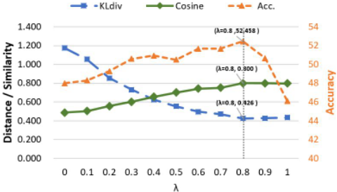
Parameter λ. The effect of parameter λ in (3) is shown in Figure 3. We use Kullbacj-Leibler divergence and cosine coefficient to demonstrate how λ influences distribution prediction. As can be seen, with the increases of λ, our multi-task framework (λ = 0.8) improves the accuracy compared with the fine-tuned VGGNet (λ = 0), which achieve 4% improvement on Emotion6. When increases from 0 to 0.6, the performance of the classification and distribution is boosted dramatically. Experiment shows the performance is stable when increases from 0.6 to 0.8, and our framework can reach a balance between the classification loss and the distribution loss in this range. Moreover, further increasing the leads to the decreasing of the accuracy since that the overusing Lsdl introduces too much ambiguity. Therefore, we set the λ = 0.8 in all our experiments for a trade-off considering, which shows that label ambiguity plays an important role in sentiment feature learning and performs well on both tasks.
4.5 Results on Single Label Dataset
Classification. We compare the proposed method with the state-of-the-art work on FI, which is the largest single label dataset in the area. The contrastive approaches include hand-crafted features based (Zhao's) and deep features based methods. Some observations can be drawn from Table 2. As expected, deep models perform better against the method employing hand-tuned features. We report the results in three popular deep architectures, i.e. AlexNet, VGGNet, and ResNet. It is consistent that when fine-tuned on the training set of FI, the performance is improved, and the proposed algorithm outperforms the state-of-the-art work in all frameworks. Since different deep architectures can capture different kinds of interests from affective images, we also ensemble the results of three models by concatenating the second fully connected layer outputs and reduce the dimension employing PCA. The results of using LIBSVM trained on the concatenated features reaches 67.48%.
λ and constraints. As summarized in Table 3, compared with the model using traditional classification loss (63.75%), our method achieves higher performance with the increasing of the weight of distribution loss. The combination of both losses (λ = 0.8, 66.21%) is also better than using distribution loss only (64.95%). Moreover, Line 4, 5, and 8 show that when generating distribution from single label, both of the proposed constraints outperform the LS method [Szegedy et al., 2016], and Constraint1 is better than the other.
5 Conclusion
In this work, we develop a multi-task deep framework to leverage the ambiguity and relationship between emotional categories for visual sentiment prediction. Extensive experiments show that our proposed method performs favorably against the state-of-the-art approaches on both distribution datasets and single label dataset.
@inproceedings{ijcai2017p456,
  title     = {Joint Image Emotion Classification and Distribution Learning via Deep Convolutional Neural Network},
  author    = {Yang, Jufeng and She, Dongyu and Sun, Ming},
  booktitle = {Proceedings of the Twenty-Sixth International Joint Conference on
               Artificial Intelligence, {IJCAI-17}},
  publisher = {International Joint Conferences on Artificial Intelligence Organization},
  editor    = {Carles Sierra},
  pages     = {3266--3272},
  year      = {2017},
  month     = {8},
  note      = {Main track},
  doi       = {10.24963/ijcai.2017/456},
  url       = {https://doi.org/10.24963/ijcai.2017/456},
}
TY - CPAPER TI - Joint Image Emotion Classification and Distribution Learning via Deep Convolutional Neural Network AU - Yang, Jufeng AU - She, Dongyu AU - Sun, Ming T2 - Proceedings of the Twenty-Sixth International Joint Conference on Artificial Intelligence, IJCAI-17 PB - International Joint Conferences on Artificial Intelligence Organization PY - 2017 SP - 3266 EP - 3272 DO - 10.24963/ijcai.2017/456 UR - https://doi.org/10.24963/ijcai.2017/456 ER -Copied
Machine-readable versions of this paper, for tools and AI agents:





