
A Decomposition Approach for Urban Anomaly Detection Across Spatiotemporal Data
Proceedings of the Twenty-Eighth International Joint Conference on Artificial Intelligence. AI for Improving Human Well-being. Pages 6043-6049.
https://doi.org/10.24963/ijcai.2019/837
Keywords
- Special Track on AI for Improving Human-Well Being: AI safety (Special Track on AI and Human Wellbeing)
Abstract
Urban anomalies such as abnormal flow of crowds and traffic accidents could result in loss of life or property if not handled properly. Detecting urban anomalies at the early stage is important to minimize the adverse effects. However, urban anomaly detection is difficult due to two challenges: a) the criteria of urban anomalies varies with different locations and time; b) urban anomalies of different types may show different signs. In this paper, we propose a decomposing approach to address these two challenges. Specifically, we decompose urban dynamics into the normal component and the abnormal component. The normal component is merely decided by spatiotemporal features, while the abnormal component is caused by anomalous events. Then, we extract spatiotemporal features and estimate the normal component accordingly. At last, we derive the abnormal component to identify anomalies. We evaluate our method using both real-world and synthetic datasets. The results show our method can detect meaningful events and outperforms state-of-the-art anomaly detecting methods by a large margin.
- [Breunig et al., 2000] Markus M Breunig, Hans-Peter Kriegel, Raymond T Ng, and Jörg Sander. Lof: identify- ing density-based local outliers. In ACM sigmod record, volume 29, pages 93-104. ACM, 2000.
- [Chandola et al., 2009] Varun Chandola, Arindam Banerjee, and Vipin Kumar. Anomaly detection: A survey. ACM computing surveys (CSUR), 41(3):15, 2009.
- [Chen et al., 2017] Longbiao Chen, Jérémie Jakubowicz, Dingqi Yang, Daqing Zhang, and Gang Pan. Fine-grained urban event detection and characterization based on tensor cofactorization. IEEE Trans. Human-Machine Systems, 47(3):380-391, 2017.
- [Cui et al., 2018] Peng Cui, Xiao Wang, Jian Pei, and Wenwu Zhu. A survey on network embedding. IEEE Transactions on Knowledge and Data Engineering, 2018.
- [Fan et al., 2016] Zipei Fan, Ayumi Arai, Xuan Song, Api- chon Witayangkurn, Hiroshi Kanasugi, and Ryosuke Shibasaki. A collaborative filtering approach to citywide human mobility completion from sparse call records. In IJCAI, pages 2500-2506, 2016.
- [Ge et al., 2011] Yong Ge, Hui Xiong, Chuanren Liu, and Zhi-Hua Zhou. A taxi driving fraud detection system. In Data Mining (ICDM), 2011 IEEE 11th International Con- ference on, pages 181-190. IEEE, 2011.
- [Gonzalez et al., 2008] Marta C Gonzalez, Cesar A Hidalgo, and Albert-Laszlo Barabasi. Understanding individual hu- man mobility patterns. nature, 453(7196):779, 2008.
- [Khezerlou et al., 2017] Amin Vahedian Khezerlou, Xun Zhou, Lufan Li, Zubair Shafiq, Alex X Liu, and Fan Zhang. A traffic flow approach to early detection of gather- ing events: Comprehensive results. ACM Transactions on Intelligent Systems and Technology (TIST), 8(6):74, 2017.
- [Lin et al., 2018] Chaoguang Lin, Qiuhan Zhu, Shunan Guo, Zhuochen Jin, Yu-Ru Lin, and Nan Cao. Anomaly de- tection in spatiotemporal data via regularized non-negative tensor analysis. Data Mining and Knowledge Discovery, pages 1-18, 2018.
- [Liu et al., 2008] Fei Tony Liu, Kai Ming Ting, and Zhi-Hua Zhou. Isolation forest. In 2008 Eighth IEEE International Conference on Data Mining, pages 413-422. IEEE, 2008.
- [Mikolov et al., 2013] Tomas Mikolov, Ilya Sutskever, Kai Chen, Greg S Corrado, and Jeff Dean. Distributed repre- sentations of words and phrases and their compositional- ity. In Advances in neural information processing systems, pages 3111-3119, 2013.
- [Pang et al., 2011] Linsey Xiaolin Pang, Sanjay Chawla, Wei Liu, and Yu Zheng. On mining anomalous patterns in road traffic streams. In International conference on advanced data mining and applications, pages 237-251. Springer, 2011.
- [Perozzi et al., 2014] Bryan Perozzi, Rami Al-Rfou, and Steven Skiena. Deepwalk: Online learning of social repre- sentations. In Proceedings of the 20th ACM SIGKDD in- ternational conference on Knowledge discovery and data mining, pages 701-710. ACM, 2014.
- [Rousseeuw and Driessen, 1999] Peter J Rousseeuw and Ka- trien Van Driessen. A fast algorithm for the mini- mum covariance determinant estimator. Technometrics, 41(3):212-223, 1999.
- [Teng et al., 2017] Xian Teng, Yu-Ru Lin, and Xidao Wen. Anomaly detection in dynamic networks using multi-view time-series hypersphere learning. In Proceedings of the 2017 ACM on Conference on Information and Knowledge Management, pages 827-836. ACM, 2017.
- [Wang et al., 2016] Youcheng Wang, Jian Xu, Ming Xu, Ning Zheng, Jinsheng Jiang, and Kaiwei Kong. A feature- based method for traffic anomaly detection. In Proceed- ings of the 2Nd ACM SIGSPATIAL Workshop on Smart Cities and Urban Analytics, page 5. ACM, 2016.
- [Witayangkurn et al., 2013] Apichon Witayangkurn, Teer- ayut Horanont, Yoshihide Sekimoto, and Ryosuke Shibasaki. Anomalous event detection on large-scale gps data from mobile phones using hidden markov model and cloud platform. In Proceedings of the 2013 ACM confer- ence on Pervasive and ubiquitous computing adjunct pub- lication, pages 1219-1228. ACM, 2013.
- [Yang and Zhou, 2011] Su Yang and Wenbin Zhou. Anomaly detection on collective moving patterns: Mani- fold learning based analysis of traffic streams. In Privacy, Security, Risk and Trust (PASSAT) and 2011 IEEE Third Inernational Conference on Social Computing (Social- Com), 2011 IEEE Third International Conference on, pages 704-707. IEEE, 2011.
- [Zhang et al., 2018] Huichu Zhang, Yu Zheng, and Yong Yu. Detecting urban anomalies using multiple spatio-temporal data sources. Proceedings of the ACM on Interactive, Mobile, Wearable and Ubiquitous Technologies, 2(1):54, 2018.
- [Zheng et al., 2014] Yu Zheng, Licia Capra, Ouri Wolfson, and Hai Yang. Urban computing: concepts, methodolo- gies, and applications. ACM Transactions on Intelligent Systems and Technology (TIST), 5(3):38, 2014.
- [Zhuang et al., 2017] Chenyi Zhuang, Nicholas Jing Yuan, Ruihua Song, Xing Xie, and Qiang Ma. Understanding people lifestyles: Construction of urban movement knowl- edge graph from gps trajectory. In IJCAI, pages 3616- 3623, 2017. IJCAI
References were extracted automatically from the PDF and may contain errors.
Full text extracted automatically from the PDF; figures, tables and equations may differ. The PDF is the version of record.
1 Introduction
Urban anomalies are typically unusual events occurring in urban environments, such as traffic congestion and unexpected crowd gathering, which may pose tremendous threats to public safety and stability if not timely handled [Zheng et al., 2014]. For example, in July 2010, a music parade in Duisburg, German, lost control of order and led to nineteen death and hundreds of injured. In December 2014, a similar tragedy happened again in Shanghai, China. Over 300,000 people crowded into the Bund of Shanghai for the New Year's fire show, which led to a severe stampede that caused 35 death and 49 injured. However, these accidents could be prevented if the urban anomalies, e.g., abnormal moving and gathering of crowds, can be detected and traced at the early stage.
Traditional anomaly detection needs a lot of human efforts, which is usually inefficient and delayed in time. In recent years, urban big data bring new methods and perspectives for urban anomaly detection. Compared with traditional methods, data-driven methods have advantages of real-time and low-cost, which make this direction with huge potential.
∗Equal contribution.
Urban anomalous events usually happen with the abnormal change of urban dynamics such as the sharp increase in crowd flows or traffic volumes, which can be detected from urban data. Urban data are produced by mobile devices or distributed sensors in cities and usually of spatial and temporal features [Gonzalez et al., 2008; Zhuang et al., 2017; Fan et al., 2016]. For instance, when people access cellular networks via their smartphones, their trajectories will be recorded. These spatiotemporal data reveal the activities of urban residents and make it possible for us to monitor the urban dynamics in real time and further identify urban anomalies by detecting abnormal fluctuations of urban dynamics.
Generally, as for the detection of urban anomalies based on spatiotemporal data-driven methods, there are the following critical challenges.
- Scarcity of anomalous events. Abnormal events rarely happen in cities. Moreover, few of them are recorded. The extreme scarcity of labeled dataset makes it difficult to detect the happening of anomalous events directly.
- Complex influence factors. The impacts of anomalous events are affected by many spatial and temporal factors. Thus, the criteria of urban anomalies may vary with different regions and time, and all those influences need to be taken into consideration when identifying anomalous events.
- Multiple data sources fusion. Different events may have impacts on different spatiotemporal data from multiple sources. Moreover, different data sources are usually in different formats such as vehicle trajectories (structured dataset), and text messages (unstructured dataset). Fusing different types of spatiotemporal data is a challenging task as well.
Considering the above challenges, we propose a decomposition framework for detecting urban anomalies across spatiotemporal data. To overcome the scarcity of anomalous events, we decompose urban data into two parts, normal component, and abnormal component. In our case, we assume the normal component is caused by regular events and can be Proceedings of the Twenty-Eighth International Joint Conference on Artificial Intelligence (IJCAI-19)
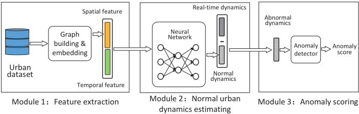
estimated by essential spatiotemporal features, while anomalous events cause the abnormal component. Unlike existing works estimating anomalous events directly, we estimate the normal component instead and derive the abnormal component using real-time dynamics to deduct the estimated normal component. Moreover, to adapt to different regions and time, we employ graph embedding technology to extract spatial features and select essential temporal features. By taking them as inputs, we use a neural network consists of three fully connected parts to fuse spatial and temporal features and estimate the normal component of urban dynamics. Also, our decomposition method is conducted on trip data of New York city from both taxis and bikes. The experiment results show that our method achieves 48.8% precision improvement compared with the best performance of baseline algorithms, which demonstrates that our framework is extendable to fuse different data sources.
The rest of this paper is organized as follows. We first introduce basic definitions and an overview of our framework in Section 2. We then describe each step of our method in details in Section 3. In Section 4, we show our datasets and experimental results. In the end, we introduce related work regarding urban anomaly detection in Section 5 and finally conclude our paper in Section 6.
2 Overview
2.1 Preliminaries
The definitions of the essential terms used in our investigated problem are shown as follows.
Definition 1 (Urban dynamics) Urban dynamics are the numerical spatial and temporal features to describe the status of an urban region during a time interval. For example, the number of people entering a region and exiting the region in one hour and the Twitter topic distribution in an area for one day [Teng et al., 2017].
Definition 2 (Urban data) Urban data are of spatial and temporal features and collected from urban sensors to describe urban dynamics. Denoting the set of urban regions as R and the set of time slots as T, thus, each instance of urban data can be denoted as a triple 〈r, t, v〉, where r ∈ R, t ∈ T , and v is a vector representing the urban dynamics in region r during time interval t. In our work, the v may contain values frommore than one data resources, like the volume of traffic flow and the density of crowds.
Definition 3 (Urban dynamic decomposition) Urban dynamics are represented by urban data. In practice, given an urban dataset S, ∀s ∈ S, s = 〈r, t, v〉, we decompose v into two parts: v = vm+va, where vm stands for the normal component of urban dynamics and va represents the abnormal component. As we assumed above, the normal component is merely depended on the spatiotemporal features which we denote as I. Therefore, vm = F(I), where F is a mapping function from the vector representing spatiotemporal features to the vector representing urban dynamics. Thus, the decomposition can be formulated as follows,
2.2 Framework
An overview of our proposed framework is shown in Figure 1. The framework is composed of three modules, feature extraction, normal urban dynamic estimating, and anomaly scoring. In the feature building module, given an urban dataset, we aim to extract the spatial-temporal features for each data point. Explicitly, we first compute region similarities based on historical data and build spatial features using the graph embedding technique. Then we select important temporal information such as time and weather to represent temporal features and concatenate spatial and temporal features together as the fused spatiotemporal feature. In the normal urban dynamic estimating module, we feed spatiotemporal features to a fully connected neural network to estimate the normal urban dynamics and obtain the anomalous urban dynamics by removing the normal component from the real dynamics. In the anomaly scoring module, the extracted abnormal component is fed into a generic anomaly detector to score the anomaly degree for a region in a time slot.
3 Methodology
In this section, we discuss our approach in detail. We first introduce the geo-embedding method to build spatial features and the strategy to select temporal features. We then present the normal urban dynamic estimating process and our designed training mechanism for the neural network. At last, we state the approach to get the final anomaly scores.
3.1 Feature Building
Spatial Features
Urban regions that are geographically close to each other or have the same city functions may have similar urban dynamics. Based on this fact, we propose a geo-embedding method that applies the Graph embedding [Cui et al., 2018; Perozzi et al., 2014] technique to extract spatial features of urban regions. We first construct a complete undirected graph, whose nodes represent regions and the edge weights are the similarity score of every two nodes. After building the graph, we apply the random walk algorithm to generate a set of trajectories for every node. Finally, we analogize nodes as words and trajectories as sentences by employing Skip-Gram model [Mikolov et al., 2013] to obtain the embedding vector for each region and use the learned vectors as spatial features. The detailed steps are illustrated as follows.
Step 1. Computing similarities of regions. Given an urban dataset S = {s0, s1, ..., sn}, where si = 〈ri, ti, vi〉. For the sake of simplicity, we use si.r to represent the ri in 〈ri, ti, vi〉. si.t and si.v are defined similarly. Denoting the set of all regions as R, for a region rm ∈ R, we define Srm = {si|si ∈ S, si.r = rm}. Then the average dynamics of region rm is computed as
where #|S| is the size of set S. Given a pair of regions rm, rn ∈ R, we define the similarity of these two regions as
where ‖v‖2 represents the l2 norm of vector v.
Step 2. Random walk. Based on the computed similarity matrix, we construct a weighted undirected graph G(V,W), where |V | = |R|. For an arbitrary pair of nodes vi, vj ∈ V , wij ∈ W refers to the weight of the edge between vertices vi and vj and is assigned as sim(ri, rj). With the graph G(V, W), we then employ the random walk method to generate a set of node trajectories T , where each trajectory is composed of a series of regions. In practice, the process starts from a random node each time and the probability moving from node u to node v is wuv/ ∑v wuv.
Step 3. Region embedding. With the trajectory set T obtained in step 2, we apply a commonly used word embedding model Skip-Gram to get the embedding vector for each region. In this process, we analogize regions as words and trajectories as sentences.
By the geo-embedding process, we obtain the spatial features that retain the similarity relations between regions. There are two advantages. First, the spatial features learning by geo-embedding take the relations between different regions into account. Hence, the knowledge from one region can be migrated to similar areas, further, improving the performance when doing the urban dynamics estimating. Second, the size of spatial features is not necessarily as large as the number of regions but can be reduced to a logarithmic length, which will significantly reduce the computational complexity.
Temporal Features
Apart from spatial features, temporal information also has a significant impact on urban dynamics. To illustrate what temporal information should be considered, we show a typical example in Figure 2 that shows the number of bikes entering a region every hour for one week. It comes from the NYC Bike dataset, which will be introduced in detail in Section 4.1.
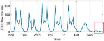
In Figure 2, there are three straightforward observations. First, the number of entering bikes reaches zero at midnight and peaks in commuting hours on weekdays. Second, the volume of bike flow during weekends is lower than that on weekdays and does not show significant peak hours. Third, the part that we mark in dashed rectangle corresponds to raining hours, when the number of bikes drops a lot compared with that on other days. According to these observations, the temporal information should include three parts, i.e., the hour in a day, the day in a week and weather. Hence, we represent the temporal features as follows,
where Ohour is a one-hot vector of length 24 that shows which hour it is in a day. Similarly, Oweekday is a one-hot vector of length 7. Oweather is also a one-hot vector shows the weather and its length depends on the weather dataset.
3.2 Normal Urban Dynamics Estimating
The main difficulty in estimating normal dynamics should be the lack of ground truth, i.e., the real value of normal urban dynamics. However, there is a simple fact that in consecutive time slots or similar regions, the normal urban dynamics should not change sharply. That is to say, the normal dynamics vm is smooth in terms of similar spatiotemporal features I. This simple fact makes it possible to learn F, i.e., the mapping relation from spatiotemporal features to normal dynamics. Given the spatiotemporal feature I, the value of F(I) should satisfy two conditions. First, since anomalous events rarely happen, F(I) should be close to the real complete urban dynamics v. Second, if I changes slightly, F(I) should not change a lot. With these two constraints, we use a neural network model with the customized loss to simulate the function F .
Figure 3 shows our neural network model. The model consists of two cascaded parts: the feature fusion part and normal urban dynamics estimation part. The first part includes FC (fully connected) network I and II, which respectively take the original spatial and temporal features as inputs. We concatenate the outputs of network I and network II together as the fused spatiotemporal feature. The second part includes FC network III, which takes the fused feature as input and outputs the estimated normal urban dynamics.
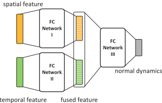
To better illustrate the definition of our customized loss function, we assume there is a pair of urban data points 〈r1, t1, v1〉 and 〈r2, t2, v2〉, and their corresponding fused features and the outputs of FC network III are 〈I1, o1〉 and 〈I2, o2〉, then the loss function L is defined as,
where Lp stands for the prediction loss, Ls refers to the smooth loss and λ is the weight for the smooth loss. The prediction loss, i.e., Lp, measures the error between network output and the real complete urban dynamic value. Thus, by reducing Lp, the network output will be pushed to be close to the real urban dynamics. Mathematically, Lp is expressed as,
where D(·) represents the mean square distance between two vectors. The smooth loss, i.e., Ls, is the ratio between output distance and input distance for the FC network III and is formulated as,
where ϵ is a small positive value. When the input features are close to each other, the value of D(I1, I2) is small, and if D(o1, o2) gets large, Ls will get large accordingly. Therefore, by reducing Ls, the output (i.e., estimated urban dynamics) is controlled to be similar when inputs (i.e., spatiotemporal features) are similar.
3.3 Anomaly Scoring
Instead of just classifying an urban scene as anomalous or not, we assign an anomaly score to each data point in the urban dataset to measure the anomaly degree of a region during a time interval. The urban dynamics of more anomaly will get higher scores. In practice, we use a general outlier detecting algorithm to obtain the score for each data point. In our case, an outlier is an observation point that is distant from other observations. Given an urban dataset S = {s0, s1, ..., sn}. For each s ∈ S, s = 〈r, t, v〉, the estimated normal component is vm and the derived abnormal component is va = v - vm. Then, the anomaly score is assigned as OScore(va), where OScore is a classical outlier detector. A lot of classical outlier detectors can be applied as OScore [Chandola et al.,
2009]. In this paper, we choose the Local Outlier Factor (LOF) [Breunig et al., 2000] algorithm.
In summary, we develop a method to decompose urban dynamics by estimating normal urban dynamics from spatiotemporal features. We construct spatiotemporal features considering the similarities among different urban regions and temporal influencing factors, which makes our method extendable to different urban datasets and complex urban environments.
4 Evaluation
4.1 Datasets and Preprocesses
To evaluate the effectiveness of our proposed framework, we conduct extensive experiments on two real-world datasets. The first dataset is the NYC taxi trip records and the second one is the NYC bike trip records 1 . The statistics of these two datasets are shown in Table 1. Besides, we crawled the weather data of New York during the data collection period from WunderGround 2 .
| Datasets | Properties | Values |
|---|---|---|
| Taxi trips | number of regions | 82 |
| duration | 14 months | |
| number of taxi trips | 194.4M | |
| Bike trips | number of stations | 750+ |
| duration | 14 months | |
| number of bike trips | 24.2M | |
| number of bikes | 16157 |
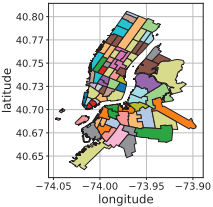
To better represent the datasets, we process the raw data in following steps. a) Divide the urban areas into small regions based on the administrative division and road networks. In Figure 4, we show the segmentation of regions in New York by colors. The number of unique regions is 82. b) Map the start and end positions into region granularity. c) Split the dataset duration into time slots of one-hour. d) For each region, compute the number of leaving trips and arriving trips during each time slot.
After the preprocesses, we can represent the NYC datasets in the format as,
where r is the region label, t stands for the time slot and v is the vector representing the number of vehicles entering and exiting the region. Each v is a 4 dimension vector [taxiin, taxiout, bikein, bikeout].
4.2 Settings and Baselines
Refer to Figure 3, we set both FC network I and II as twolayer networks and FC network III as a three-layer network. λ in (5) is set to 10-3 in the experiments. To evaluate the effectiveness of our framework, we compare our methods with four baselines:
1 http://www.nyc.gov/html/tlc/html/about/trip record data.shtml
2 https://www.wunderground.com
- Elliptic envelope (EE): EE algorithm [Rousseeuw and Driessen, 1999] fits the data points with an elliptic envelope and uses Mahalanobis distances to measure the outlyingness. For this method, we use the entire urban dynamics as inputs.
- Isolation forest (IF): IF algorithm [Liu et al., 2008] constructs binary trees based on the attributes of data points, in which an outlier is closer to the root. It computes the outlyingness based on the results from a number of trees.
- Local outlier factor (LOF): LOF algorithm [Breunig et al., 2000] compares the local density of a data point to the to the local densities of its neighbors. The points that have a substantially lower density than their neighbors are considered to be outliers. In experiments, we directly feed the full urban dynamics data into the LOF algorithm to get the anomaly score.
- Ours without geo-embedding (Ours No G.): In this algorithm, we adopt our method without geo-embedding and use one-hot vectors to encodes different regions as the spatial features.
4.3 Synthetic Anomaly Detection
We first evaluate our proposed framework using synthetic datasets. In this experiment, we generate synthetic datasets based on the real-world datasets and then test our method with injected anomalous events.
Synthetic Data Generation
We first generate a one-week standard data that does not have anomalies and then extend the dataset by repeating along the time axis and randomly inject anomalous events. In practice, we compute the one-week average of the real urban dataset as the standard data. For each data point 〈r, t, v〉, we aggregate the dynamic value v into the mod(t, 168) time slot, 168 = 24(h)×7(day), for region r and then compute the mean value.
Next, we repeat the dataset along the timeline and add 10% noises by multiplying the original value with a factor sampled from a normal distribution with mean 1 and variance 0.1. To simulate the real world situations, we also add 10% rainy and snowy weather, when the urban dynamics are reduced by 50%, where we determine the weather partition and effects based on observations on real dataset. Finally, to inject anomalous events, we multiply the urban dynamics by w when assuming that there is an anomalous event. Here, w is the weight parameter.
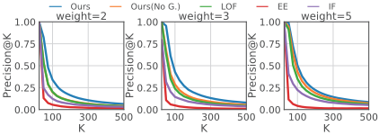
- (a) Precision@K on synthetic dataset
- (b) Recall@K on synthetic dataset
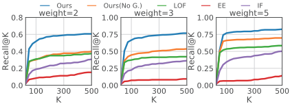
Figure 5: Top-k precision and recall on synthetic dataset.
Results for Synthetic Dataset
By the steps described above, we generate a synthetic dataset of 20 weeks. We use the data of the first 19 weeks for training and the data of the last week for testing. We use Mean Average Precision (MAP), precision at top-k positions (Precision@k), and recall at top-k positions (Recall@k) as evaluation metrics.
The MAPs of our method and four baselines are shown in Table 2. We set the weight of anomalous events w = {2, 3, 5} and compute the average MAP of 5 independent experiments for each algorithm under each setting. In all cases, our method significantly outperforms baseline algorithms. In average, the MAP of our method is 48.8% higher than the best MAP scores of baselines. Notably, compared with LOF which detects anomalies directly from undecomposed urban dynamics, our method reaches 65.8% precision improvement. The results demonstrate that the abnormal urban dynamics obtained by our decomposition approach can act as direct evidence to reveal abnormal events. Compared with 'Ours (No G.)' merely using one-hot vectors as spatial features, adopting geo-embedding brings 52.9% MAP improvement, which proves that similarity information among locations helps to improve the detection performance.
We also show the top-k precision and top-k recall in Figure 5, where K varies from 1 to 500. When K is small, all methods have precision close to 1. When K get larger, the precision of baseline methods drops sharply while the precision of our method decays slowly and consistently keeps the best. Similarly, our method also reaches a significantly better recall with K getting larger.
We also study the sensitivity of our model to the parameter λ. We set λ = {0, 10-4 , 10-3 , 10-2 , 10-1 , 1} and run our model on the synthetic dataset. With fixing other experiment settings, the MAP scores under different λ settings are shown in Table 3. When λ changes from 0 (smooth loss is ignored) to 10-4 , there is an apparent increase of MAP score. When λ gets larger than 10-3 , the constraint of smooth loss is too strong, and the MAP score drops again. The best performance is achieved when λ = 10-3 .
| Algorithms | Weights | ||
|---|---|---|---|
| w=2 | w=3 | w=5 | |
| IF | 0.090 | 0.162 | 0.254 |
| EE | 0.066 | 0.048 | 0.068 |
| LOF | 0.298 | 0.363 | 0.532 |
| Ours (No G.) | 0.278 | 0.417 | 0.656 |
| Ours | 0.506 | 0.663 | 0.772 |
| λ | 0 | 0.0001 | 0.001 | 0.01 | 0.1 | 1 |
| MAP | 0.421 | 0.529 | 0.531 | 0.488 | 0.453 | 0.281 |
4.4 Real World Anomaly Detection
The real world event detection experiment is conducted on the NYC datasets. We collect 20 events in New York with accurate time and locations 3 in two months from November 2017 to December 2017 as ground truth. For example, {Christmas Tree Lighting, 2017/12/1 18:00-20:00, Bryant Park} are the description, time and location of one recorded event. We mark the 10% most anomalous data points reported by each method as anomalies and check how many of the collected events are hit. Here, we consider an anomalous event is hit if the detected anomaly spatially and temporally overlaps with the reported event.
The experiment results for the real world datasets are shown in Table 4. With the anomalous component obtained by our decomposition method, 14 out of the 20 events are detected, while the LOF method merely hits three events. Meanwhile, the performance of other baselines is also worse than ours.
| Methods | IF | EE | LOF | Ours(No G.) | Ours |
|---|---|---|---|---|---|
| Hits | 8 | 8 | 3 | 8 | 14 |
| Hit ratio | 40% | 40% | 15% | 40% | 70% |
In conclusion, our method outperforms baselines on both synthetic and real-world datasets. The results show that our decomposition framework significantly improves the anomaly detection accuracy and the geographic correlations extracted by our geo-embedding method also improves the performance.
5 RelatedWork
The general anomaly detection task aims to detect data points that deviate significantly from the others in a dataset. Lots of algorithms have been proposed towards this problem [Chandola et al., 2009]. The existing works that specifically focus on urban anomaly detection can be categorized into three groups: feature based, matrix based and statistical methods.
3 www.nycinsiderguide.com
Feature-based methods extract human designed features from urban datasets and then apply classical outlier detecting algorithms to identify anomalies. Simple physical features such as speed [Wang et al., 2016] and distance [Ge et al., 2011] are widely used in traffic anomaly detection. Some other works are based on high-level features. For example, Zhang et al. [Zhang et al., 2018] computed the similarity of urban dynamics of different regions within a time window and detect anomalous regions based on the similarity changing rate. However, in these methods the features are constructed based on either spatial information or temporal information while our method fuses spatial and temporal features together.
By representing urban data as matrices or tensors, techniques such as tensor decomposition are used to process urban data. For example, Lin et al. [Lin et al., 2018] applied the tensor decomposition method to represent urban data with combinations of basic patterns, then detect anomalies based on pattern weights. Chen et al. [Chen et al., 2017] proposed a similar method but design a co-factorization algorithm that decomposes a mobility matrix and check-in tensor together. [Yang and Zhou, 2011] combined the LLE and PCA algorithms to detect anomalies from traffic flow matrix. In these methods, the regions are considered independently, while our method takes the spatial correlations among regions into consideration.
Statistical models are also commonly used in urban anomaly detection. For example, the Hidden Markov Model is used to model the status transition of urban dynamics [Yang and Zhou, 2011; Witayangkurn et al., 2013] and the change of a low probability is considered caused by anomalous events. Khezerlou et al. [Khezerlou et al., 2017] utilized the Likelihood Ratio Test (LRT) method to detect gathering events based on traffic flow. Pang et al. [Pang et al., 2011] also extended the LRT method to discover traffic anomalies. However, the influence of some random factors such as weather is not considered in statistical methods.
6 Conclusion
In this paper, we proposed a decomposition method to detect urban anomalies based on urban big data. We first selected information to build the temporal feature and designed a geo-embedding method to learn the spatial feature of regions. We then estimated the normal component using neural networks based on spatiotemporal features and derived the abnormal component accordingly. Finally, we employed the LOF method to detect anomalies by assigning an anomaly score to each data point. We conducted extensive experiments on both real-world and synthetic datasets to evaluate our method. The experiment results demonstrated the superiority of our approach.
Acknowledgments
This research has been supported in part by project 16214817 from the Research Grants Council of Hong Kong, project FP805 from HKUST, and the 5GEAR project from the Academy of Finland.
@inproceedings{ijcai2019p837,
  title     = {A Decomposition Approach for Urban Anomaly Detection Across Spatiotemporal Data},
  author    = {Zhang, Mingyang and Li, Tong and Shi, Hongzhi and Li, Yong and Hui, Pan},
  booktitle = {Proceedings of the Twenty-Eighth International Joint Conference on
               Artificial Intelligence, {IJCAI-19}},
  publisher = {International Joint Conferences on Artificial Intelligence Organization},
  editor    = {Sarit Kraus},
  pages     = {6043--6049},
  year      = {2019},
  month     = {8},
  note      = {AI for Improving Human Well-being},
  doi       = {10.24963/ijcai.2019/837},
  url       = {https://doi.org/10.24963/ijcai.2019/837},
}
TY - CPAPER TI - A Decomposition Approach for Urban Anomaly Detection Across Spatiotemporal Data AU - Zhang, Mingyang AU - Li, Tong AU - Shi, Hongzhi AU - Li, Yong AU - Hui, Pan T2 - Proceedings of the Twenty-Eighth International Joint Conference on Artificial Intelligence, IJCAI-19 PB - International Joint Conferences on Artificial Intelligence Organization PY - 2019 SP - 6043 EP - 6049 DO - 10.24963/ijcai.2019/837 UR - https://doi.org/10.24963/ijcai.2019/837 ER -Copied
Machine-readable versions of this paper, for tools and AI agents:





