
Taming Decentralized POMDPs: Towards Efficient Policy Computation for Multiagent Settings
Proceedings of the Eighteenth International Joint Conference on Artificial Intelligence. Pages 705-710.
Abstract
The problem of deriving joint policies for a group of agents that maximize some joint reward function can be modeled as a decentralized partially observable Markov decision process (POMDP). Yet, despite the growing importance and applications of decentralized POMDP models in the multiagents arena, few algorithms have been developed for efficiently deriving joint policies for these models. This paper presents a new class of locally optimal algorithms called "Joint Equilibriumbased search for policies (JESP)". We first describe an exhaustive version of JESP and subsequently a novel dynamic programming approach to JESP. Our complexity analysis reveals the potential for exponential speedups due to the dynamic programming approach. These theoretical results are verified via empirical comparisons of the two JESP versions with each other and with a globally optimal brute-force search algorithm. Finally, we prove piece-wise linear and convexity (PWLC) properties, thus taking steps towards developing algorithms for continuous belief states.
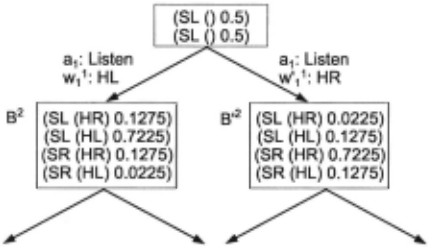
- SR (HR) 0.1275) (SR (HL) 0.0225) 8' 2 (SL (HR) 0.0225) (SL (HL) 0.1275) (SR (HR) 0.7225) (SR (HL) 0.1275)
- [Bernstein eta!., 2000] D. Bernstein, S. Zilberstein, and N. Immerman. The complexity of decentralized control ofMDPs. In UAI, 2000.
- [Boutilier, 1996] C. Boutilier. Planning, learning & coor- dination in multiagent decision processes. In TARK-96, 1996.
- [Cassandra eta/., 1997] A. Cassandra, M. Littman, and N. Zhang. Incremental pruning: A simple, fast, ex- act method for partially observable markov decision pro- cesses. In UAI, 1997.
- MUL TIAGENT SYSTEMS [Chades eta/., 2002] I. Chades, B. Scherrer, and F. Charpil- let. A heuristic approach for solving decentralized-pomdp: Assessment on the pursuit problem. In SAC, 2002.
- [Kaelbling eta/., 1998] L. Kaelbling, M. Littman, and A. Cassandra. Planning and acting in partially observable stochastic domains. Artificial Intelligence, 101 , 1998.
- [Monahan, 1982] G. Monahan. A survey of partially observ- able markov decision processes: Theory, models and algo- rithms. ManagementScience, 101(1):1-16,January 1982.
- [Papadimitriou and Tsitsiklis, 1987] C. Papadimitriou and J. Tsitsiklis. Complexity of markov decision pro- cesses. Mathematics of Operatios Research, 12(3):441 - 450, 1987.
- [Peshkin eta/., 2000] L. Peshkin, N. Meuleau, K. E. Kim, and L. Kaelbling. Learning to cooperate via policy search. In UAI, 2000.
- [Pynadath and Tambe, 2002] D. Pynadath and M. Tambe. The communicative multiagent team decision problem: Analyzing teamwork theories and models. lAIR, 2002.
- [Sondik, 1971] Edward J. Sondik. The optimal control of partially observable markov processes. Ph.D. Thesis, Stan- ford, 1971.
- [Xuan eta!., 2001] P. Xuan, V. Lesser, and S. Zilberstein. Communication decisions in multiagent cooperation. In Agents-0 1, 2001 .
References were extracted automatically from the PDF and may contain errors.
Full text extracted automatically from the PDF; figures, tables and equations may differ. The PDF is the version of record.
1 Introduction
As multiagent systems move out of the research lab into crit ical applications such as multi-satellite control, researchers need to provide high-performing, robust multiagent designs that are as nearly optimal as feasible. To this end, researchers have increasingly resorted to decision-theoretic models as a framework in which to formulate and evaluate multiagent de signs. Given a group of agents, the problem of deriving sep arate policies for them that maximize some joint reward can be modeled as a decentralized POMDP (Partially Observable Markov Decision Process). In particular, the DEC-POMDP (Decentralized POMDP) [Bernstein eta/., 2000] and MTDP (Markov Team Decision Problem [Pynadath and Tambe, 2002]) are generalizations of a POMDP to the case where there are multiple, distributed agents basing their actions on their separate observations. These frameworks allow a vari ety of multiagent analysis. Of particular interest here, they allow us to formulate what constitutes an optimal policy for a multiagent system and in principle derive that policy.
However, with a few exceptions, effective algorithms for deriving policies for decentralized POMDPs have not been developed. Significant progress has been achieved in efficient single-agent POMDP policy generation algorithms [Mona han, 1982; Cassandra eta/., 1997; Kaelbling eta/. , 1998]. However, it is unlikely such research can be directly car ried over to the decentralized case. Finding optimal poli cies for decentralized POMDPs is NEXP-complete [Bern stein eta/., 2000]. In contrast, solving a POMDP is PSPACE complete [Papadimitriou and Tsitsiklis, 1987]. As Bernstein et al. [2000] note, this suggests a fundamental difference in the nature of the problems. The decentralized problem can not be treated as one of separate POMDPs in which individ ual policies can be generated for individual agents because of possible cross-agent interactions in the reward, transition or observation functions. (For any one action of one agent, there may be many different rewards possible, based on the actions that other agents may take.) In some domains, one possibility is to simplify the nature of the policies considered for each of the agents. For example, Chades et al. [2002] restrict the agent policies to be memoryless (reactive) poli cies. Further, as an approximation, they define the reward function and the transition function over observations instead of over states thereby simplifying the problem to solving a multi-agent MDP [Boutilier, 1996]. Xuan et a/. [200 1] de scribe how to derive decentralized MDP (not POMDP) poli cies from a centralized MDP policy. Their algorithm, which starts with an assumption of full communication that is grad ually relaxed, relies on instantaneous and noise free commu nication. Such simplifications reduce the applicability of the approach and essentially side-step the question of solving de centralized POMDPs. Peshkin et al. [2000] take a different approach by using gradient descent search to find local op timum finite-controllers with bounded memory. Their algo rithm finds locally optimal policies from a limited subset of policies, with an infinite planning horizon, while our algo rithm finds locally optimal policies from an unrestricted set of possible policies, with a finite planning horizon.
Thus, there remains a critical need for new efficient algorithms for generating optimal policies in distributed POMDPs. In this paper, we present a new class of algorithms for solving decentralized POMDPs, which we refer to as Joint Equilibrium-based Search for Policies (JESP). JESP iterates through the agents, finding an optimal policy for each agent assuming the policies of the other agents are fixed. The it eration continues until no improvements to the joint reward is achieved. Thus JESP achieves a local optimum similar to a Nash Equilibrium. We discuss Exhaustive-JESP which uses exhaustive search to find the best policy for each agent. Since this exhaustive search for even a single agent's policy can be very expensive, we also present DP-JESP which im proves on Exhaustive-JESP by using dynamic programming to incrementally derive the policy. We conclude with sev eral empirical evaluation that contrast JESP against a glob ally optimal algorithm that derives the globally optimal pol icy via a full search of the space of policies. Finally, we prove piece-wise linear and convexity (PWLC) properties, thus tak ing steps towards developing algorithms for continuous initial belief states.
2 Model
We describe the Markov Team Decision Prob lem (MTDP) [Pynadath and Tambe, 2002] frame work in detail here to provide a concrete illustra tion of a decentralized POMDP model. However, other decentralized POMDP models could poten tially also serve as a basis [Bernstein et a!., 2000; Xuan eta!., 2001].
Given a team of n agents, an MTDP [Pynadath and Tambe, 2002] is defined as a tuple: (S, A, P, n, 0, R). S is a finite set of world states {1, 2, ... , m }. A = x 1<=i<=nA;, where At, ... , An, are the sets of action for agents I to n. A joint action is represented as (at, ... , an). P(s;, (a1, ... , an) , s 1 ), the transition function, represents the probability of the current state is s 1, if the previous state is s; and the previous joint action is (at, ... , an) . nl ' ... 'nn are the set of observations for agents 1 to n. 0 ( s, ( a1, .. . , an) , w) , the observation function, represents the probability of joint observation w, if the current state is s and the previous joint action is (a1, ... , an). The agents receive a single, immediate joint reward R(s, at, . . . , an) which is shared equally.
Practical analysis using models like MTDP often assume that observations of each agent is independent of each other's observations. Thus the observation function can be expressed as O(s,(a1, ... ,an),w) = Ot(s,(at, ... ,an),wt) · ... · On(s , (a1, ... ,an) ,wn).
Each agent i chooses its actions based on its local policy, 1r;, which is a mapping of its observation history to actions. Thus, at time t , agent i will perform action 7r;(wf) where wf = w}' .. . 'wf. 7r = ( 7rl' . . . '7r n) refers to the joint policy of the team of agents. The important thing to note is that in this model, execution is distributed but planning is central ized. Thus agents don't know each other's observations and actions at run-time but they know each other's policies.
3 Example Scenario
For illustrative purposes it is useful to consider a familiar and simple example, yet one that is capable of bringing out key difficulties in creating optimal policies for MTDPs. To that end, we consider a multiagent version of the classic tiger problem used in illustrating single agent POMDPs[Kael bling eta!., 1998] and create an MTDP ((S,A,P,n, O,R)) for this example. In our modified version, two agents are in a corridor facing two doors:"left" and "right". Behind one door lies a hungry tiger and behind the other lies un told riches but the agents do not know the position of ei ther. Thus, S = {SL, SR}, indicating behind which door the tiger is present. The agents can jointly or individually open either door. In addition, the agents can independently listen for the presence of the tiger. Thus, At = A2 = {'OpenLeft', 'OpenRight', 'Listen'}. The transition func tion P , specifies that every time either agent opens one of the doors, the state is reset to SL or SR with equal proba bility, regardless of the action of the other agent, as shown in Table 1. However, if both agents listen, the state remains unchanged. After every action each agent receives an obser vation about the new state. The observation function, 0 1 or 0 2 (shown in Table 2) will return either H L or H R with dif ferent probabilities depending on the joint action taken and the resulting world state. For example, if both agents listen and the tiger is behind the left door (state is SL), each agent receives the observation H L with probability 0.85 and H R with probability 0.15.
| I Actionffransition | I SL ~ SL | SL ~ SR | SR ~ SR | SR -t |
|---|---|---|---|---|
| <OpenRight, *> | 0.5 | 0.5 | 0.5 | 0.5 |
| <OpenLeft,*> | 0.5 | 0.5 | 0.5 | 0.5 |
| <*,OpenLeft> | 0.5 | 0.5 | 0.5 | 0.5 |
| < *, OpenRight> | 0.5 | 0.5 | 0.5 | 0.5 |
| <Listen,Listen> | 1.0 | 0.0 | 1.0 | 0.0 |
| Action | State | HL | HR |
|---|---|---|---|
| <Listen,Listen> | SL | 0.85 | 0.15 |
| <Listen,Listen> | SR | 0.15 | 0.85 |
| <OpenRight, *> | * | 0.5 | 0:5 |
| <OpenLeft,*> | * | 0.5 | 0.5 |
| <*,OpenLeft> | * | 0.5 | 0.5 |
| <*,OpenRight> | * | 0.5 | 0.5 |
If either of them opens the door behind which the tiger is present, they are both attacked (equally) by the tiger (see Table 3). However, the injury sustained if they opened the door to the tiger is less severe if they open that door jointly than if they open the door alone. Similarly, they receive wealth which they share equally when they open the door to the riches in proportion to the number of agents that opened that door. The agents incur a small cost for performing the 'Listen' action.
Clearly, acting jointly is beneficial (e.g., At = A2 = 'OpenLeft') because the agents receive more riches and sus tain less damage by acting together. However, because the agents receive independent observations (they do not share observations), they need to consider the observation histories of the other agent and what action they are likely to perform.
| Action/State | SL | SR |
|---|---|---|
| <OpenRight,OpenRight> | +20 | -50 |
| <Open Left, OpenLeft> | -50 | +20 |
| <OpenRight,OpenLeft> | -100 | -100 |
| <OpenLeft,OpenRight> | -100 | -100 |
| <Listen,Listen> | -2 | -2 |
| <Listen,OpenRight> | +9 | -101 |
| <OpenRight,Listen> | +9 | -101 |
| <Listen,OpenLeft> | -101 | +9 |
| <OpenLeft,Listen> | -101 | +9 |
We also consider consider another case of the reward func tion, where we vary the penalty for jointly opening the door to the tiger (See Table 4).
| Action/State | SL | SR |
|---|---|---|
| <OpenRight,OpenRight> | +20 | 0 |
| <Open Left, OpenLeft> | -50 | +20 |
| < OpenRight, OpenLeft> | -100 | -100 |
| <Open Left, OpenRight> | -100 | -100 |
| <Listen,Listen> | -2 | -2 |
| <Listen,OpenRight> | +9 | -101 |
| <OpenRight,Listen> | +9 | -101 |
| <Listen,OpenLeft> | -101 | +9 |
| <OpenLeft,Listen> | -101 | +9 |
4 Optimal Joint Policy
When agents do not share all of their observations, they must instead coordinate by selecting policies that are sensitive to their teammates' possible beliefs, of which each agent's en tire history of observations provides some information. The problem facing the team is to find the optimal joint policy, i.e. a combination of individual agent policies that produces behavior that maximizes the team's expected reward.
One sure-fire method for finding the optimal joint policy is to simply search the entire space of possible joint policies, evaluate the expected reward of each, and select the policy with the highest such value. To perform such a search, we must first be able to determine the expected reward of a joint policy. We compute this expectation by projecting the team's execution over all possible branches on different world states and different observations. We present here the 2-agent ver sion of this computation, but the results easily generalize to arbitrary team sizes. At each time step, we can compute the expected value of a joint policy, 1r = (1r1, 1r2), for a team starting in a given state, st' with a given set of past observa tions, wf and w~, as follows:
At each time step, the computation of v; performs a summation over all possible world states and agent observations, so the time complexity of this algorithm is 0 ((fS[·[fh[·[fhif). The overall search performs this computation for each and every possible joint pol icy. Since each policy specifies different actions over pos sible histories of observations, the number of possible policies for an individual agent i is 0 (1Aii ' IA~~--/). The number of possible joint policies for n agents is thus 0 ( (I A* 1 1 1~g-~ I) n)' where A* and n* correspond to the largest individual action and observation spaces, respec tively, among the agents. The time complexity for find ing the optimal joint policy by searching this space is thus: 0 ( (lA* 1 1 1°~~--~~) n · (lSI · ID* ln)T)
5 Joint Equilibrium-based Search for Policies
Given the complexity of exhaustively searching for the op timal joint policy, it is clear that such methods will not be successful when the amount of time to generate the policy is restricted. In this section, we will present algorithms that are guaranteed to find a locally optimal joint policy. We refer to this category of algorithms as "JESP" (Joint Equilibrium Based Search for Policies). Just like the solution in Section 4, the solution obtained using JESP is a Nash equilibrium. In particular it is a locally optimal solution to a partially ob servable identical payoff stochastic game(POIPSG) [Peshkin eta/. , 2000]. The key idea is to find the policy that maxi mizes the joint expected reward for one agent at a time, keep ing the policies of all the other agents fixed. This process is repeated until an equilibrium is reached (local optimum is found). The problem of which optimum the agents should se lect when there are multiple local optima is not encountered since planning is centralized.
5.1 Exhaustive approach(Exhaustive-JESP)
The algorithm below describes an exhaustive approach for JESP. Here we consider that there are n cooperative agents. We modify the policy of one agent at a time keeping the poli cies of the other n - 1 agents fixed. The function best Policy, returns the joint policy that maximizes the expected joint reward, obtained by keeping n - 1 agents' policies fixed and exhaustively searching in the entire policy space of the agent whose policy is free. Therefore at each itera tion, the value of the modified joint policy will always either increase or remain unchanged. This is repeated until an equi librium is reached, i.e. the policies of all n agents remains unchanged. This policy is guaranteed to be a local maximum since the value of the new joint policy at each iteration is non decreasing.
Algorithm 1 EXHAUSTIVE-JESP() I: prev +- random joint policy, conv +- 0 2: while conv =f. n - 1 do 3: fori +- 1 ton do 4: fix policy of all agents except i 5: policySpace +- list of all policies fori 6: new+- bestPolicy(i,policySpace,prev) 7: if new. value = prev. value then 8: conv+-conv + 1 9: else I 0: prev +- new, conv +- 0 II : ifconv = n -1 then 12: break 13: return newThe best policy cannot remain unchanged for more than n - 1 iterations without convergence being reached and in the worst case, each and every joint policy is the best policy for at least one iteration. Hence, this algorithm has the same worst case complexity as the exhaustive search for a globally optimal policy. However, it could do much better in practice as illustrated in Section 6. Although the solution found by this algorithm is a local optimum, it may be adequate for some applications. Techniques like random restarts or simulated annealing can be applied to perturb the solution found to see if it settles on a different higher value.
The exhaustive approach to Steps 5 and 6 of the Exhaustive-JESP algorithm enumerates and searches the entire policy space of a single agent, i. There are 0 (JA;I'IA~~---; 1 ) such policies, and evaluating each incurs
a time complexity of 0 ((lSI · IDIT)). Thus, using the ex
haustive approach incurs an overall time complexity in Steps
complexity cost in each and every pass through the JESP algorithm, a faster means of performing the bestPolicy function call of Step 6 would produce a big payoff in overall efficiency. We describe a dynamic programming alternative to this exhaustive approach for doing JESP next.
5.2 Dynamic Programming (DP-JESP)
If we examine the single-agent POMDP literature for inspi- . ration, we find algorithms that exploit dynamic programming to incrementally construct the best policy, rather than simply search the entire policy space [Monahan, 1982; Cassandra et a/., 1997; Kaelbling eta/., 1998]. These algorithms rely on a principle of optimality that states that each sub-policy of an overall optimal policy must also be optimal. In other words, if we have a T -step optimal policy, then, given the history over the first t steps, the portion of that policy that covers the last T - t steps must also be optimal over the remaining T- t steps. In this section, we show how we can exploit an anal ogous optimality property in the multiagent case to perform more efficient construction of the optimal policy within our JESP algorithm.
To support such a dynamic-programming algorithm, we must define belief states that summarize an agent's history of past observations, so that they allow the agents to ignore the actual history of past observations, while still supporting construction of the optimal policy over the possible future. In the single-agent case, a belief state that stores the distri bution, B!ingle = Pr( st Jwt), is a sufficient statistic, because the agent can compute an optimal policy based on B!ingle without having to consider the actual observation sequence, c;;t [Sondik, 1971].
In the multiagent case, an agent faces a complex but nor mal single-agent POMDP if the policies of all other agents are fixed. However, B!ingle, is not sufficient, because the agent must also reason about the action selection of the other agents and hence on the observation histories of the other agents. Thus, at each time t, the agent i reasons about the tuple d = (s t -t ) h -t - ( -t -t -t -t) . ,w#i, were w#i- w1 , ... ,wi_1,wi+1 , ... ,wn IS the joint observation histories of all the agents except i . By treating e: to be the state of the agent i at timet, we can define the transition function and observation function for the single agent POMDP for agent i as follows:
where 1r #i = ( rri, ... , rr!-u rr!+l, ... , rr~) is the joint policy for all agents except i.
We now define the novel multiagent belief state for an agent i given the distribution over the initial state, b( s) = Pr(S 1 = s):
In other words, when reasoning about an agent's policy in the context of other agents, we maintain a distribution over e:, rather than simply the current state. Figure 1 shows different belief states B 1 , B 2 and B' 2 for agent 1 in the tiger domain. For instance, B 2 , shows probability distributions over ei. In e~ = (SL, (H R)), (H R) is the history of agent 2's observa tions while SL is the current state. Section 5.3 demonstrates how we can use this multiagent belief state to construct a dy namic program that incrementally constructs the optimal pol icy for agent i.
5.3 The Dynamic Programming Algorithm
Following the model of the single-agent value-iteration al gorithm, our dynamic program centers around a value func tion over a T -step finite horizon. For readability, this sec tion presents the derivation for the dynamic program in the two-agent case; the results easily generalize to the n-agent case. Having fixed the policy of agent 2, our value function Vi(Bt), represents the expected reward that the team will re~ ceive when agent I follows its optimal policy from the t-th step onwards when starting with a current belief state, Bf . We start at the end of the time horizon (i.e., t = T), and then work our way back to the beginning. Along the way, we con struct the optimal policy by maximizing our value function over possible action choices:
We can define the action value function, Vt 1 , recursively:
The first term in equation 6 refers to the expected immediate reward, while the second term refers to the expected future re ward. Bf+l is the belief state updated after performing action a1 and observing wf+ 1 . In the base case, t = T, the future reward is 0, leaving us with:
The calculation of expected immediate reward breaks down as follows:
Thus, we can compute the immediate reward using only the agent's current belief state and the primitive elements of our given MTDP model (See Section 2).
Computation of the expected future reward (the second term in Equation 6) depends on our ability to update agent I 's belief state from Bf to Bf+l in light of the new observa tion, wf+l For example, in Figure I, the belief state B 1 is updated to B' 2 on performing action a1 and receiving obser-. 11 nr d · I vatwn w1 . vve now enve an a gorithm for performing such an update, as well as computing the remaining Pr(wiB,a) term from Equation 6. The initial belief state based on the distribution over initial state, b, is:
For ~~+1 =. (St+t, (w~,w~+ 1 )), the updated Bf+1(e~+ 1 ) is obtamed usmg EquatiOns 2 and 3 and Bayes Rule and is given as follows:
We treat the denominator of Equation I 0 (i.e., Pr(wf+ 1 IBL at)) as a normalizing constant to bring the sum of the numerator over all ei to be I . This result also enters into our computation of future expected reward in the second term of Equation 6. Thus, we can compute the agent's new belief state (and the future expected reward and the overall value function, in tum) using only the agent's current belief state and the primitive elements of our given MTDP model. Having computed the overall value function, vt, we can also extract a form of the optimal policy, 1r1 , that maps observation histories into actions, as required by Equations 8 and IO.
Algorithm 2 presents the pseudo-code for our overall dy namic programming algorithm. Lines 1- 6 generate all of the belief states reachable from a given initial belief state, b(s) = Pr(S 1 = s) . Since there is a possibly unique belief state for every sequence of actions and observations by agent I, there are 0 ((IA1I·Ifld)T) reachable belief states. This reachability analysis uses our belief update procedure (Algo rithm 3 ), which itself has time complexity 0 (IS 1 2 102 1 t+l) when invoked on a belief state at time t. Thus, the over all reachability analysis phase has a time complexity of O((ISI 2 (IAll·lfl1l·lfl21)T). Lines 7-22 perform the heart of our dynamic programming algorithm, which also has a time complexity of O((S 2 (IA1I·Ifld ·lf221)T). Lines 2327 translate the resulting value function into an agent policy defined over observation sequences, as required by our al gorithm (i.e., the 1r2 argument). This last phase has a lower time and space complexity, O(ISI 2 If!dT · lf22 lr), than our other two phases, since it considers only optimal actions for agent I. Thus, the overall time complexity of our algorithm is 0 (S 2 (IA1I·Ifl1l · lfl21)T) . The space complexity of the resulting value function and policy is essentially the product of the number of reachable belief states and the size of our belief state representation: 0 (ISI(IA1I·Iflll ·lfl21)T) .
5.4 Piecewise Linearity and Convexity of Value Function
Algorithm 2 computes a value function over only those be lief states that are reachable from a given initial belief state which is a subset of all possible probability distributions ove; S t d -t ... d . . an w 2 . 10 use ynam1c programmmg over the entire set, we must show that our chosen value function is piecewise lin:ar and convex (PWLC). Each agent is faced with solving a smgle agent POMDP is the policies of all other agents is fixed as shown in Section 5.2. Sondik [I97I] showed that the value function for a single agent POMDP is PWLC. Hence the value function in Equation 5 is PWLC. Thus, in addition
Algorithm 2 OPTIMALPOLICYDP(b, 1r2, T)
I : reachable(O) ~ { b} 2: for t ~ 1 to T do 3: for all Bt- l E reachable(t- 1) do 4: reachable(t) ~ 0 5: for all a1 E At,Wt E Ot do 6: reachable(t) f!- UPDATE(Bt-I,at,wt) 7: fort ~ T downto 1 do 8: for all Bt E reachable(t) do 9: Vt(Bt) ~ -oo 10: for all at EAt do II: Vt 1 (Bt) ~ 0 12: for all s E S,w2 E 0~ do {Equation 8} 13: Vt 1 (Bt) t- Bt(s,w2) · R (s, (at, 1r2(w2))) 14: ift < T then {Compute future reward} 15: for all Wt E 01 do 16: prob ~ 0 17: for all st, st+ 1 E S, w2 E 0~ do 18: act~ (ai,1r2(w2)) 19: prob t.. Bt ( st, w2) · P( st, act, st+l) Ot (st+l, act, Wt) 20: ~a 1 (Bt) t.. prob litH (UPDATE(Bt, all Wt)) {Equation 6} 21 : if~a 1 (Bt) > vt(Bt) then 22: vt(Bt) ~ ~al (Bt) 23: for all Wt E Of do 24: B 0 ~ b 25: fort~ 1 toT do 26: Bt ~ UPDATE( Bt-l, 7rt (wt(l. .. (t- 1)]), wt(t]) 27: 1r1 (wt [1 . .. t]) ~ arg maxa 1 ~a 1 (Bt) 28: return 1ftAlgorithm 3 UPDATE(Bt, at, wt) for all st+l E S, w2 E 0~+1 do Bt+t(st+t,w2) ~ o act ~ (at, 1r2 (w2 [1. .. t])) for all st E S do {Equation 10} Bt+l (st+l, w2) t.. P(st, act, st+l) 02(st+l' act, w2[t + 1]) normalize Bt+l ( st+l, wt) return Bt+l Bt(st ,w2[1 ... t]) Ot ( st+t, act, Wt)to supporting the more efficient dynamic programming of Al gorithm 2, our novel choice of belief state space and value function can potentially support a dynamic programming al gorithm over the entire continuous space of possible belief states.
6 Experimental Results
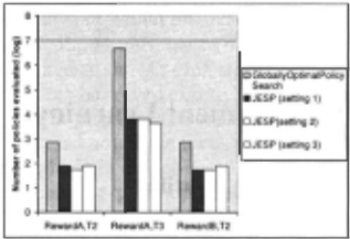
In this section, we perform an empirical comparison of the algorithms described in Sections 4 and 5 using the Tiger Sce nario (See Section 3) in terms of time and performance. Fig ure 2, shows the results of running the globally optimal al gorithm and the Exhaustive JESP algorithm for two different reward functions (Tables 3 and 4. Finding the globally op timal policy is extremely slow and is doubly exponential in the finite horizon, T and so we evaluate the algorithms only for finite horizons of 2 and 3. We ran the JESP algorithm for 3 different randomly selected initial policy settings and compared the performance of the algorithms in terms of the number of policy evaluations (on Y-axis using log scale) that were necessary. As can be seen from this figure, for T = 2 the JESP algorithm requires much fewer evaluations to arrive at an equilibrium. The difference in the run times of the glob ally optimal algorithm and the JESP algorithm is even more apparent when T = 3. Here the globally optimal algorithm performed > 4 million policy evaluations while the JESP al gorithm did < 7000 evaluations. For the reward function A, JESP succeeded in finding the globally optimal policies for both T = 2 (expected reward= -4) and 3 (expected reward = -6). However, this is not always the case. Using reward function B for T = 2, the JESP algorithm sometimes settles on a locally optimal policy (expected reward= -4) that is different from the globally optimal policy (expected reward = 20). However, when random restarts are used, the globally optimal reward can be obtained.
Based on Figure 2, we can conclude that the exhaustive JESP algorithm performs better than an exhaustive search for the globally optimal policy but can some times settle on a pol icy that is only locally optimal. This could be sufficient for problems where the difference between the locally optimal policy's value and the globally optimal policy's value is small and it is imperative that a policy be found quickly. Alterna tively,the JESP algorithm could be altered so that it doesn't get stuck in a local optimum via random restarts.
Table 5 compares presents experimental results from com parison of exhaustive JESP with our dynamic programming approach (DP-JESP). These results, also from the tiger do main, show run-time in milliseconds (ms) for the two algo rithms with increasing horizon. DP-JESP is seen to obtain significant speedups over exhaustive-JESP. For time horizon of2 and 3 DP-JESP run time is essentially 0 ms, compared to the significant run times ofExhaustive-JESP. As we increased the horizon to > 3, we could not run exhaustive-JESP at all; while DP-JESP could be easily run up to horizon of 7.
7 Summary and Conclusion
With the growing importance of decentralized POMDPs in the multiagents arena, for both design and analysis, it is crit ical to develop efficient algorithms for generating joint policies. Yet, there is a significant lack of such efficient algo rithms. There are three novel contributions in this paper to address this shortcoming. First, given the complexity of the exhaustive policy search algorithm- doubly exponential in the number of agents and time - we describe a class of algorithms called "Joint Equilibrium-based Search for Poli cies" (JESP) that search for a local optimum rather than a global optimum. In particular, we provide detailed algorithms for Exhaustive JESP and dynamic programming JESP(DP JESP). Second, we provide complexity analysis for DP-JESP, which illustrates a potential for exponential speedups over ex haustive JESP. We have implemented all of our algorithms, and empirically verified the significant speedups they pro vide. Third, we provide a proof that the value function for individual agents is piece-wise linear and convex (PWLC) in their belief states. This key result could pave the way to a new family of algorithms that operate over continuous be lief states, increasing the range of applications that can be at tacked via decentralized POMDPs, and is now a major issue for our future work.
| Method |
| Exhaustive-JESP |
|---|
| DP-JESP |
Acknowledgments
We thank Piotr Gmytrasiewicz for discussions related to the paper. This research was supported by NSF grant #0208580 and DARPA award no. F30602-98-2-0108.
@inproceedings{ijcai2003p103,
  title     = {Taming Decentralized POMDPs: Towards Efficient Policy Computation for Multiagent Settings},
  author    = {Nair, Ranjit and Tambe, Milind and Yokoo, Makoto and Pynadath, David V. and Marsella, Stacy},
  booktitle = {Proceedings of the Eighteenth International Joint Conference on
               Artificial Intelligence, {IJCAI-03}},
  publisher = {International Joint Conferences on Artificial Intelligence},
  editor    = {Georg Gottlob and Toby Walsh},
  pages     = {705--710},
  year      = {2003},
  url       = {https://ijcai.org/proceedings/2003/103},
}
TY - CPAPER TI - Taming Decentralized POMDPs: Towards Efficient Policy Computation for Multiagent Settings AU - Nair, Ranjit AU - Tambe, Milind AU - Yokoo, Makoto AU - Pynadath, David V. AU - Marsella, Stacy T2 - Proceedings of the Eighteenth International Joint Conference on Artificial Intelligence, IJCAI-03 PB - International Joint Conferences on Artificial Intelligence PY - 2003 SP - 705 EP - 710 UR - https://ijcai.org/proceedings/2003/103 ER -Copied
Machine-readable versions of this paper, for tools and AI agents:





