
Fast Algorithm for Affinity Propagation
Proceedings of the Twenty-Second International Joint Conference on Artificial Intelligence. Pages 2238-2242.
Abstract
Affinity Propagation is a state-of-the-art clustering method recently proposed by Frey and Dueck. It has been successfully applied to broad areas of computer science research because it has much better clustering performance than traditional clustering methods such as k-means. In order to obtain high quality sets of clusters, the original Affinity Propagation algorithm iteratively exchanges real-valued messages between all pairs of data points until convergence. However, this algorithm does not scale for large datasets because it requires quadratic CPU time in the number of data points to compute the messages. This paper proposes an efficient Affinity Propagation algorithm that guarantees the same clustering result as the original algorithm after convergence. The heart of our approach is (1) to prune unnecessary message exchanges in the iterations and (2) to compute the convergence values of pruned messages after the iterations to determine clusters. Experimental evaluations on several different datasets demonstrate the effectiveness of our algorithm.
- [Chang and Zheng, 2009] Xueping Chang and Zhonglong Zheng. Laplacian discriminant projection based on affin- 8 http://www.geonames.org/export/wikipedia-webservice.html ity propagation. In Int. Conf. Artificial Intelligence and Computational Intelligence (AICI), pages 313-321, 2009. Link
- [Crandall et al., 2009] David J. Crandall, Lars Backstrom, Daniel Huttenlocher, and Jon Kleinberg. Mapping the world's photos. In Int. World Wide Web Conf. (WWW), pages 761-770, 2009.
- [Dueck and Frey, 2007] Delbert Dueck and Brendan J. Frey. Non-metric affinity propagation for unsupervised image categorization. In IEEE Int. Conf. Computer Vision (ICCV), pages 1-8, 2007.
- [Frey and Dueck, 2007] Brendan J. Frey and Delbert Dueck. Clustering by passing messages between data points. Sci- ence, 315:2007, 2007.
- [Hu et al., 2010] Rong Hu, Brian Mac Namee, and Sarah Jane Delany. Off to a good start: Using clus- tering to select the initial training set in active learning. In Florida Artificial Intelligence Research Society Conf. (FLAIRS), 2010.
- [Jain et al., 1999] Anil K. Jain, M. Narasimha Murty, and Patrick J. Flynn. Data clustering: A review. ACM Comput. Surv., 31(3):264-323, 1999.
- [Jia et al., 2008] Yangqing Jia, Jingdong Wang, Changshui Zhang, and Xian-Sheng Hua. Finding image exemplars using fast sparse affinity propagation. In ACM Int. Conf. Multimedia (ACM MM), pages 639-642, 2008.
- [Kennedy and Naaman, 2008] Lyndon S. Kennedy and Mor Naaman. Generating diverse and representative image search results for landmarks. In Int. World Wide Web Conf. (WWW), pages 297-306, 2008.
- [Liu et al., 2009] Zhiyuan Liu, Peng Li, Yabin Zheng, and Maosong Sun. Clustering to find exemplar terms for keyphrase extraction. In Conf. Empirical Methods in Natu- ral Language Processing (EMNLP), pages 257-266, 2009.
- [Tong et al., 2008] Hanghang Tong, Christos Faloutsos, and Jia-Yu Pan. Random walk with restart: fast solutions and applications. Knowl. Inf. Syst., 14(3):327-346, 2008.
- [Zha et al., 2009] Zheng-Jun Zha, Linjun Yang, Tao Mei, Meng Wang, and Zengfu Wang. Visual query suggestion. In ACM Int. Conf. Multimedia (ACM MM), pages 15-24, 2009.
References were extracted automatically from the PDF and may contain errors.
Full text extracted automatically from the PDF; figures, tables and equations may differ. The PDF is the version of record.
1 Introduction
Cluster analysis is an important component of scientific and industrial data analysis, and many clustering methods have been proposed [Jain et al., 1999]. When a set of data points is given, clustering assigns each data point into a group (cluster). By using clustering, we can extract representative examples from the dataset or discover the structures present in the raw data.
Recently, Frey and Dueck proposed a novel clustering method, named Affinity Propagation [Frey and Dueck, 2007]. Affinity Propagation recursively transmits real-valued messages between all pairs of data points until message values converge. And it determines a set of clusters and their representative data points called 'exemplars', based on the converged message values. Affinity Propagation has a number of noteworthy advantages. For instance, (1) it achieves much lower clustering error than existing clustering methods such as k-means clustering [Jain et al., 1999], (2) it can support similarities that are not symmetric or do not satisfy the triangle inequality, and (3) it is deterministic, i.e., its clustering results do not depend on initialization, unlike most clustering methods such as k-means. Therefore, it has been successfully used in many applications in various disciplines such as initial training set selection in active learning [Hu et al., 2010], keyphrase extraction [Liu et al., 2009], image clustering [Jia et al., 2008] [Dueck and Frey, 2007], representative image extraction [Zha et al., 2009], and supervised dimensionality reduction [Chang and Zheng, 2009].
Although Affinity Propagation has been receiving a lot of attention for use in many applications, one of the most important research issues is its speed, especially for large scale datasets [Jia et al., 2008]. This is because the original Affinity Propagation algorithm requires quadratic CPU time in the number of data points to compute the messages. For resolving this issue, Jia et al. recently proposed FSAP, a fast algorithm for Affinity Propagation [Jia et al., 2008]. However, their algorithm achieves its efficiency at the expense of clustering result accuracy; its clustering results are not the same as those of the original Affinity Propagation algorithm. Sacrificing clustering accuracy makes it difficult to realize truly effective applications.
In this paper, we propose an efficient clustering algorithm for Affinity Propagation that gives the same clustering result as the original algorithm after convergence. In order to reduce computation cost without loss of clustering accuracy, the proposal (1) prunes unnecessary message exchanges between data pairs in the iterations to compute the convergence values, and (2) computes the convergence values of pruned messages from those of unpruned messages. Moreover, our algorithm does not require users to set any inner-parameters, unlike FSAP. FSAP has a specific inner-parameter that must be carefully set if the clustering results are not to be negatively impacted. We conduct evaluation experiments on several different datasets to compare our algorithm against existing algorithms. The results demonstrate the superiority of our algorithm. It is much faster than the existing algorithms while it guarantees exactness of the clustering results. This confirms the practicality of our algorithm for real world applications. With our method, many applications can be processed more efficiently.
The remainder of this paper is organized as follows. Section 2 gives a brief review of the original Affinity Propagation algorithm and FSAP. Section 3 introduces the main ideas and details of our algorithm. Section 4 reviews the results of our experiments. Section 5 provides our conclusions.
| Symbol | Definition |
|---|---|
| N | Number of data points |
| T | Number of iterations |
| s[i, j] | Similarity between data point i and j |
| r[i, j] | Responsibility between data point i and j |
| a[i, j] | Availability between data point i and j |
| ρ[i, j] | Propagating responsibility between data point i and j |
| α[i, j] | Propagating availability between data point i and j |
| λ | Damping factor, 0 ≤ λ < 1 |
2 Preliminary
In this section, we briefly review the original Affinity Propagation algorithm proposed by Frey and Dueck [Frey and Dueck, 2007], as well as FSAP [Jia et al., 2008], a state-ofthe-art fast algorithm for Affinity Propagation. Table 1 lists the main symbols and their definitions.
2.1 Affinity Propagation
Affinity Propagation is a clustering algorithm that identifies a set of 'exemplars' that represents the dataset [Frey and Dueck, 2007]. The input of Affinity Propagation is the pair-wise similarities between each pair of data points, s[i, j](i, j = 1, 2, . . . ,N ) 1 . Any type of similarities is acceptable, e.g. negative Euclidean distance for real valued data and Jaccard coefficient for non-metric data, thus Affinity Propagation is widely applicable.
Given similarity matrix s[i, j], Affinity Propagation attempts to find the exemplars that maximize the net similarity, i.e. the overall sum of similarities between all exemplars and their member data points. The process of Affinity Propagation can be viewed as a message passing process with two kinds of messages exchanged among data points: responsibility and availability. Responsibility, r[i, j], is a message from data point i to j that reflects the accumulated evidence for how well-suited data point j is to serve as the exemplar for data point i. Availability, a[i, j], is a message from data point j to i that reflects the accumulated evidence for how appropriate it would be for data point i to choose data point j as its exemplar. All responsibilities and availabilities are set to 0 initially, and their values are iteratively updated as follows to compute convergence values:
where λ is a damping factor introduced to avoid numerical oscillations, and ρ[i, j] and α[i, j] are, we call, propagating responsibility and propagating availability, respectively. ρ[i, j] and α[i, j] are computed by the following equations:
1 s[i, i] for each data point is called preference and impacts the number of clusters.
That is, messages between data points are computed from the corresponding propagating messages. The exemplar of data point i is finally defined as:
As described above, the original algorithm requires O(N 2 T ) time to update massages, where N and T are the number of data points and the number of iterations, respectively. This incurs excessive CPU time, especially when the number of data points is large. Therefore, a fast Affinity Propagation algorithm is demanded as pointed out in [Jia et al., 2008].
2.2 FSAP
For resolving the computation time issue of the original Affinity Propagation algorithm, Jia et al. recently proposed FSAP [Jia et al., 2008]. One promising idea for improving the speed of Affinity Propagation is to reduce the number of message values that need to be computed. FSAP aims to reflect this idea as follows. The first stage of FSAP constructs a K-nearest neighbor graph. If data point i is among the K data points that have the largest similarity with data point j, then data point i and j are connected by an edge, otherwise not. Since FSAP performs message transmissions on the Knearest neighbor graph, too many exemplars (at least N/K) might be generated. Therefore, in order to merge multiple exemplars into one cluster, the second stage adds further edges based on the following three criteria:
- If data point i is the exemplar of data point j, then data point i and j are connected by an edge;
- For two data points i and j, if there exists two data points m and n that take data point i and j as their exemplar, respectively, and data point m and n are K-nearest neighbor to each other, and so data point i and j are connected by an edge; and
- For two data points i and j, if they are connected by criterion 2, then all data points that choose data point i as exemplar are connected to data point j, and vise versa.
After convergence, the exemplar of data point i is finally determined by Equation (4).
They showed that their approach is much faster than the original algorithm described in Section 2.1. However, FSAP is based on heuristic ideas, i.e., the linked edges are determined based on K-nearest neighbor approximation and heuristic criteria. Therefore, FSAP does not guarantee the same result as the original Affinity Propagation algorithm. As we will show in Section 4, this fact seriously degrades the clustering accuracy. Our algorithm presented in this paper is faster than FSAP while it still theoretically guarantees the exactness of the clustering results after convergence.
3 Proposed method
In this section, we present our fast Affinity Propagation algorithm which gives the same clustering result as the original algorithm after convergence. First, we give an overview of the ideas underlying the proposed algorithm and then a full description. We also give some theoretical analyses of its performance.
3.1 Ideas
In order to improve running speed, we construct a sparse graph structure G = [V,E] where node set V and edge set E correspond to data points and a part of the messages between any two of the data points, respectively. This allows us to compute the message values efficiently. This is because the propagating responsibility and propagating availability that need to be computed are limited to those on existing edges. However, one may easily raise the following questions: how can we identify a set of necessary edges that yields the same clustering result as the original algorithm?
We can identify the edges whose convergence values do not need to be computed by estimating their upper and lower bounds. Based on this idea, we can construct a sparse graph that has no unnecessary edges. Moreover, as we describe later, the convergence values of pruned (unnecessary) messages can be computed from that of unpruned (necessary) messages. Therefore, after the iterations, we can compute the convergence values of pruned messages. This is our answer to the question. As a result, we can efficiently obtain the same clustering result as the original algorithm.
These new ideas provide a further advantage. Our upper/lower bound estimation does not need any user-defined inner-parameters, whereas FSAP has one parameter, K, for determining the K-nearest neighbor graph. The value of K impacts the clustering result. That is, our algorithm is user friendly.
3.2 Approach
We first describe how to construct the sparse graph structure, and give some theoretical highlights of the sparse graph structure. And then, we detail our clustering algorithm.
Sparse graph structure
We reduce the number of messages between data points in the iterations in order to compute the convergence values at low cost. To realize efficient computation, we construct graph G = [V,E] where node set V consists of data points. We prune unnecessary messages by estimating upper/lower values of convergence values. We show the following lemma of convergence message values:
Lemma 1 (Convergence message) After convergence, message values of responsibility and availability are r[i, j] = ρ[i, j] and a[i, j] = α[i, j], respectively.
This lemma implies that if the Affinity Propagation algorithm converges, its convergence values can be computed from the definition of propagating messages (Equation (2) and (3)).
By utilizing the above lemma, upper/lower values of convergence messages can be obtained from just pair-wise similarities. Formally, the following equations give upper/lower values of convergence message values:
Definition 1 (Upper/lower bound) The following definitions give upper/lower bounding estimations a[i, j], r[i, j], and a[i, j] for convergence messages:
Note that a[i, j] can be computed just from pair-wise similarities s[i, j](i, j = 1, 2, . . . ,N ) since r[j, j] = s[j, j] - maxk̸=j {s[j, k]} (Equation (2)). In addition, r[i, j] and a[i, j] can be computed from a[i, j] and r[i, j], respectively. Therefore, we do not need any iterations to compute these upper/lower bounding values.
We show the following lemmas to introduce the upper/lower properties of a[i, j], r[i, j], and a[i, j].
Lemma 2 (Upper/lower bound) For any node pairs i and j in graph G, a[i, j] ≤ a[i, j], r[i, j] ≥ r[i, j], and a[i, j] ≥ a[i, j] hold after convergence.
Proof. We first prove that a[i, j] ≤ a[i, j]. From Lemma 1, a[i, j] = α[i, j] holds after convergence. If i ̸=j, then a[i, j] ≥ min{0, r[j, j]} = a[i, j] holds since ∑k̸=i,jmax{0, r[k, j]} ≥ 0. If i = j, then a[i, j] ≤ a[i, j] holds since ∑k̸=imax{0, r[k, i]} ≥ 0. We next prove that r[i, j] ≥ r[i, j]. This is obvious from Lemma 1, Equation (2), and a[i, j] ≤ a[i, j]. We finally prove that a[i, j] ≥ a[i, j]. This is similarly obvious given Lemma 1, Equation (3), and r[i, j] ≥ r[i, j]. ✷
We construct the sparse graph structure by pruning unnecessary messages by using upper/lower bound estimations. Formally, we obtain the edge between node i and j as follows:
Definition 2 (Sparse graph) The sparse graph G, where node set V consists of data points, has an edge between node i and j if and only if:
We introduce the following two lemmas to describe the property of our graph structure:
Lemma 3 (Convergence availability values) For any node pair i and j, convergence values of availabilities can be exactly computed just from the convergence responsibilities that satisfy r[i, j] ≥ 0.
Proof. From Lemma 1, a[i, j] = α[i, j] holds after convergence. If r[i, j] < 0 holds for a pair, the responsibility of the pair does not affect the values of ∑k̸=i,jmax{0, r[k, j]} and ∑k̸=imax{0, r[k, j]} in Equation (3) after convergence. ✷
Algorithm 1 Proposed algorithm
Input: pair-wise similarities Output: exemplars of each data point 1: for each data point pair [i, j] do 2: compute a[i, j], r[i, j], and a[i, j] by Equation (5-7); 3: end for 4: for each data point pair [i, j] do 5: if r[i, j]≥0 or a[i, j]+s[i, j]≥maxk̸= j{a[i, k]+s[i, k]}then 6: link data point pair [i, j]; 7: end if 8: end for 9: for t = 1 to T do 10: for each linked data point pair [i, j] do 11: update r[i, j] and a[i, j] by Equation (1); 12: end for 13: end for 14: for each unlinked data point pair [i, j] do 15: compute r[i, j] = ρ[i, j] and a[i, j] = α[i, j]; 16: end for 17: for each data point i do 18: compute exemplar by Equation (4); 19: end forLemma 4 (Convergence responsibility values) For any node pair i and j, convergence values of responsibilities can be exactly computed just from the convergence availabilities that satisfy a[i, j] + s[i, j] ≥ maxk̸=j {a[i, k] + s[i, k]}.
Proof. From Lemma 1, r[i, j] = ρ[i, j] holds after convergence. If i ̸=j, r[i, j] = s[i, j] - maxk̸=j {a[i, k] + s[i, k]} holds from Equation (2) after convergence. Since maxk̸=j {a[i, k] + s[i, k]} ≥ maxk̸=j {a[i, k] + s[i, k]} holds, if maxk̸=j {a[i, k] + s[i, k]} > a[i, j] + s[i, j] holds for node pair i and j, then maxk̸=j {a[i, k] + s[i, k]} > a[i, j] + s[i, j] holds for the node pair. Therefore, the availability values of the pair does not affect the values of responsibilities. If i = j, responsibilities can be computed just from pair-wise similarities (see Equation (2)). ✷
From Lemma 3 and 4, we introduce the following lemma:
Lemma 5 (Convergence in the sparse graph structure)
For any node pair i and j, convergence values of messages can be exactly obtained by computing convergence values of edge messages in sparse graph G.
Proof. This is obvious given Lemma 1, 3, and 4. ✷ Lemma 5 provides our algorithm with the property of clustering results which is the same as the original Affinity Propagation algorithm.
Clustering algorithm
Algorithm 1 is the full description of our algorithm. We first compute the upper/lower values of convergence messages by Definition 1 (lines 1-3), and then construct the graph structure by Definition 2 (lines 4-8). Since we can compute the convergence message values of all data point pairs from those of graph edges (Lemma 5), we iteratively update the message values of graph edges to compute convergence values (lines 9-13). Then we compute convergence message values of unlinked data point pairs after the iterations (lines 1416). These values can be computed by propagating messages after the iterations (Lemma 1). We finally compute exemplars for all data points (lines 17-19).
Note that, our algorithm itself does not require any userdefined inner-parameters. Thus it provides to the user with a simple solution to Affinity Propagation with enhanced clustering speed.
3.3 Theoretical analyses
We provide theoretical analyses with regard to the clustering results and computation cost of our algorithm. Let M be the number of edges in the graph. That is M = |E|.
Theorem 1 (Clustering results) After convergence, the clustering results of our algorithm are same as those of the original Affinity Propagation.
Proof. It is obvious fromLemma 5. ✷Theorem 2 (Computation cost) Our algorithm requires O(N 2 + MT ) time to obtain exemplars for all data points.
Proof. In the clustering process of our algorithm, we first compute the upper/lower values of convergence messages of all data point pairs, and construct the graph structure. These procedures require O(N 2 ) time since the upper/lower values can be computed just from pair-wise similarities. Then, we iteratively compute the convergence message values for all edges in the graph, which needs O(MT ) time. We finally compute convergence message values of unlinked edges and exemplars for all data points which require O(N 2 - M ) and O(N 2 ) time, respectively. Therefore, the computation cost of our algorithm is O(N 2 + MT ). ✷
4 Experimental evaluation
We conducted evaluation experiments to confirm the effectiveness of our algorithm. In these evaluations, we compare our algorithm to the original Affinity Propagation algorithm [Frey and Dueck, 2007] and FSAP [Jia et al., 2008].
Our experiments will demonstrate that:
- Efficiency: Our algorithm outperforms the original algorithm and FSAP in terms of computation time (Section 4.1).
- Exactness: Unlike FSAP, our algorithm yields the same clustering result as the original algorithm (Section 4.2).
- Applicability: Case-studies on real world datasets shows that our algorithm and FSAP output different clustering results, and that the results of our algorithm are reasonable (Section 4.3). That is, our algorithm can be a better alternative for the original algorithm.
In this section, Proposed and Original represent the results of our algorithm and the original algorithm, respectively. FSAP is tested under several different values of K. FSAP(5%), FSAP(10%), and FSAP(20%) refer to the results of FSAP gained with K values of 0.05N, 0.1N, and 0.2N, respectively. We iteratively computed responsibilities and availabilities a thousand times to obtain convergence values. We set the damping parameter, λ, to 0.5.
In the experiments, we used the following three datasets of different application domains that have different characteristics each other:
- Geo: This dataset was collected by downloading geotagged photographs from Flickr 2 using the site's public API 3 . The crawled data consists of 10, 000 photographs and their associated geotag data. All photos were taken in the central area of New York City, the United States between January 1st, 2006 and June 31st, 2009. Geo location of each photo is represented as its longitude and latitude (x, y). Similarity between photo i and j is the negative Euclidean distance.
- Dictionary 4 : This dataset was taken from word network in FOLDOC 5 . FOLDOC is a famous on-line, searchable, encyclopedic dictionary of computing subjects. Similarity between term i and j is computed by random walk with restart [Tong et al., 2008] where relevance from term i to j is the frequency with which term j is used to describe the meaning of term i. The number of terms is 13, 356.
- Traffic 6 : This dataset contains loop sensor measurements of the Freeway Performance Measurement System. This loop sensor dataset was collected in Los Angeles from April 10th, 2005 to October 1st, 2005 (5 minute count aggregates). We extracted 10, 000 sequences from the sensor measurements. Similarity between sequence i and j is taken as the negative Euclidean distance.
All experiments were conducted on a Linux quad 3.33 GHz Intel Xeon server with 32GB of main memory. We implemented all algorithms using GCC.
4.1 Efficiency
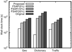
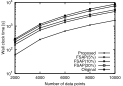
We evaluated the clustering performance of each algorithm through wall clock time. Figure 1 shows the results. We also show the scalability of each algorithm in Figure 2; this figure shows the wall clock time as a function of the number of data points. We show only the result of Geo in Figure 2 due to space limitations.
These figures show that our algorithm is significantly faster than the original algorithm under all conditions examined. Specifically, our algorithm is more than 30 times faster than the original algorithm. As described in Section 2, the original algorithm requires O(N 2 T ) while our algorithm requires O(MT ) time (see Theorem 2) in the iterations. And, as Precision Recall shown in Table 2, there are very few edges in our sparse graph (i.e., M ≪ N 2 ) 7 . This is because a significant number of messages are pruned by our upper and lower bounding strategies. Therefore, our algorithm is an extremely efficient variant of the original algorithm.
2 http://www.flickr.com/
3 http://maps.google.com/
4 http://vlado.fmf.uni-lj.si/pub/networks/data/dic/foldoc/foldoc.zip
5 http://foldoc.org/
6 http://archive.ics.uci.edu/ml/datasets/Dodgers+Loop+Sensor
| Algorithm | Data set | ||
|---|---|---|---|
| Geo | Dictionary | Traffic | |
| Proposed | 10,009,002 | 2,799,319 | 10,034,228 |
| Original | 100,000,000 | 178,382,736 | 100,000,000 |
And our algorithm is much faster than FSAP whose efficiency depends on the value of inner-parameter K as shown in the results. FSAP is a two-stage approach and it needs iterations in each stage (see Section 2.2). Therefore, our algorithm is faster than FSAP.
4.2 Exactness
One major advantage of our algorithm is that it guarantees the same clustering result as that of the original algorithm after convergence. However, this raises the following simple question: how successful is FSAP in providing the same clustering results?
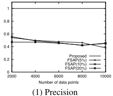
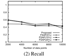
To answer this question, we compared the exemplars extracted by our algorithm and FSAP to those extracted by the original algorithm. As the measures of accuracy, we used precision and recall. Precision is the fraction of exemplars by our algorithm that are match those of the original algorithm. And recall is the fraction of exemplars extracted by the original algorithm that were successfully extracted by our algorithm. We used Geo as the dataset in these experiments.
Figure 3-(1) and 3-(2) show the precision and recall, respectively. As we can see from Figure 3-(1) and 3-(2), the precision and recall of our algorithm are always 1. Because our algorithm is theoretically designed to compute convergence message values exactly, our algorithm does not sacrifice clustering accuracy. FSAP, on the other hand, has lower precision and recall. This is because FSAP determines edges based on heuristic ideas (see Section 2.2). The results shown in Figure 1, 2, and 3 confirm that our algorithm is superior to the original algorithm in terms of speed, and to FSAP in both of accuracy and speed.
7 Our additional experiments confirmed that a data pair which has higher similarity value has a higher chance to have an edge.
4.3 Application example
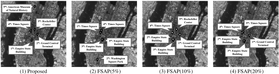
To demonstrate the impact of our algorithm on real world applications, we give some examples of its clustering performance on Geo. The clustering of a geo-tagged photo dataset is regarded as the detection of popular landmarks that are frequently taken into photos, and this is recognized as a key process in many geo-location oriented applications such as geo-referenced image browsing [Crandall et al., 2009] and landmark image search [Kennedy and Naaman, 2008].
Figure 4 shows exemplars of the top 5 (largest) clusters extracted by our algorithm and FSAP. To find a place name for a given exemplar (longitude/latitude), we used a public reverse geocoding tool based on georeferenced Wikipedia articles 8 . All algorithms detected famous landmarks such as the Empire State Building, Times Square, and Grand Central Terminal. However, FSAP detected the same landmark more than once. For instance, FSAP(5%) redundantly detected the Empire State Building (3rd and 5th) and Times Square (1st and 4th). On the other hand, all popular landmarks extracted by our algorithm were different from each other. The result of our algorithm is reasonable, and is consistent with our intuition. Note that the result of our algorithm equals that of the original algorithm. These results imply that our algorithm can be another option for the research community for clustering large datasets.
5 Conclusions
This paper proposed an efficient clustering algorithm for Affinity Propagation that gives the same clustering result as the original algorithm after convergence. Our algorithm is based on two ideas: (1) it prunes unnecessary message exchanges in the iterations, and (2) it computes the convergence values of pruned messages from those of unpruned messages. Experiments show that our algorithm can achieve efficient clustering without sacrificing clustering accuracy. Affinity Propagation is fundamental for many applications in various disciplines. The proposed solution allows many applications to be processed more efficiently, and helps to improve the effectiveness of future applications.
@inproceedings{ijcai2011p373,
  title     = {Fast Algorithm for Affinity Propagation},
  author    = {Fujiwara, Yasuhiro and Irie, Go and Kitahara, Tomoe},
  booktitle = {Proceedings of the Twenty-Second International Joint Conference on
               Artificial Intelligence, {IJCAI-11}},
  publisher = {AAAI Press/International Joint Conferences on Artificial Intelligence},
  editor    = {Toby Walsh},
  pages     = {2238--2242},
  year      = {2011},
  month     = {7},
  doi       = {10.5591/978-1-57735-516-8/IJCAI11-373},
  url       = {https://doi.org/10.5591/978-1-57735-516-8/IJCAI11-373},
}
TY - CPAPER TI - Fast Algorithm for Affinity Propagation AU - Fujiwara, Yasuhiro AU - Irie, Go AU - Kitahara, Tomoe T2 - Proceedings of the Twenty-Second International Joint Conference on Artificial Intelligence, IJCAI-11 PB - AAAI Press/International Joint Conferences on Artificial Intelligence PY - 2011 SP - 2238 EP - 2242 DO - 10.5591/978-1-57735-516-8/IJCAI11-373 UR - https://doi.org/10.5591/978-1-57735-516-8/IJCAI11-373 ER -Copied
Machine-readable versions of this paper, for tools and AI agents:





