Adaptive Budget Allocation for Maximizing Influence of Advertisements

1 Introduction

Suppose an advertiser wishes to maximize the influence on customers, but has limited budgets to allocate across media (e.g., webpages, television, or newspapers). The main question, called the budget allocation problem, is how to select media considering budget constraints such that the largest fraction of customers can be influenced; that is, how can a budget achieve the maximum reach?

The main difficulty behind the budget allocation problem is the complex dynamic of influence from media to customers. This dynamic has been investigated in the framework of the influence maximization problem, which was first introduced by Domingos and Richardson [2001; 2002]. A seminal work by Kempe, Kleinberg, and Tardos [2003] formulated the influence maximization problem in the framework of submodularity. The submodularity concept represents a certain diminishing marginal return property in discrete settings. Kempe et al. showed that the expected number of customers influenced by media is represented by a submodular set function. On the basis of this observation, they proved an approximation guarantee of a polynomial-time greedy algorithm for the influence maximization problem.

These studies on the influence maximization problem motivated the work of Alon, Gamzu, and Tennenholtz [2012], who formulated the budget allocation problem in the bipartite influence model as another combinatorial optimization problem and provided a provable approximation algorithm. There was difficulty in expressing their problem setting using submodular functions because submodularity is usually defined for combinations of objects whereas budget allocations are assignments of budgets to media. However, Soma et al. [2014] showed that the problem setting of Alon et al. can also be expressed in the framework of submodularity. They utilized submodularity functions over an integer lattice, which are more general than submodular set functions.

Despite these developments, the previous studies on the budget allocation problem have a crucial limitation. In their settings, advertisers have to assign their entire budget at once at the beginning of the process. However, in reality, advertisers routinely adjust their strategy when they see changes in the dynamic or when something unexpected happens. For example, in the US presidential campaign of 2012, both Obama and Romney spent half a billion dollars for TV ads [The Washington Post, 2012]. In particular, they invested huge amounts of money in "swing" states. For these states, both campaigns changed their strategy for TV ads every day, according to their polls (i.e., either gaining momentum or not). In this case, momentum changed frequently, and the dynamic was a deciding factor in their strategy. Hence, both the campaigns changed their strategy adaptively every day. In this paper, we are motivated by this observation. We aim to consider adaptive strategies to address the budget allocation problem.

Adaptivity has been already considered in the framework of submodularity. Golovin and Krause [2011b] defined a concept of adaptive submodularity, and showed that a greedy adaptive algorithm has a theoretical approximation guarantee if the objective function is adaptive monotone submodular. After their initial work, numerous studies further investigated algorithms for optimization problems with adaptive submodular functions [Golovin and Krause, 2011a; Gabillon et al., 2013; 2014; Gotovos et al., 2015], as well as their applications [Golovin et al., 2010; Chen and Krause, 2013; Chen et al., 2014; Deshpande et al., 2014; Krause et al., 2014; Chen et al., 2015]. Because the model of Golovin and Krause contains the adaptive setting of Kempe et al. [2003], adaptive strategies have been already analyzed in the influence maximization problem. However, adaptive strategies for the budget allocation problem have not been captured by their model. Thus, we need to formulate a new concept of adaptive submodularity that can model the budget allocation problem.

1.1 Contributions

In this paper, we consider adaptive strategies in the budget allocation problem in the bipartite influence model introduced by Alon et al. [2012]. To this end, we define adaptive submodularity of functions over integer lattices, which is a new concept that extends both the adaptive submodularity given by Golovin and Krause [2011b] and submodularity over integer lattice used in Soma et al. [2014] (see Section 3.3). This concept captures the objective function in the adaptive version of the budget allocation problem. Hence we obtain a good adaptive strategy for the budget allocation problem by designing a strategy for maximizing an adaptive submodular function over an integer lattice.

In many variants of the submodular maximization problems, the greedy algorithms achieve good performance both in practice and in theory. Thus we analyze the performance of greedy adaptive algorithms for maximizing adaptive monotone submodular functions over integer lattices. For our problem, a greedy strategy repeats allocating a certain amount of budget to a medium so that the increase of the influence per allocated budget is maximized. In our setting, the strategy is given a new feedback when it allocates a unit amount of budget. It is natural to update the strategy each time a new feedback is given. We call such a strategy sensitive greedy strategy. On the other hand, an insensitive greedy strategy ignores feedbacks until a certain proportion of a budget has been allocated to a media. Surprisingly, we can show both theoretically and empirically that several typical sensitive greedy strategies are inferior even to the non-adaptive algorithms. Our proposal algorithms are sort of insensitive greedy strategies.

More specifically, we present the following two variations of the insensitive greedy algorithms.

• ÷ An algorithm outputs a budget allocation that achieves (1-1◁e)-approximation. That is, its expected objective value is at least (1 - 1◁e) times that achieved by arbitrary adaptive algorithms. The allocation may violate the budget constraints by a factor of at most two; however, its expected cost is at most the given budget upper limit. (see Theorem 3)
• ÷ Another algorithm outputs a budget allocation of an approximation ratio (e - 1)◁(2e). The allocation is guaranteed to satisfy the budget constraints. (see Theorem 4)

Alon et al. [2012] showed that a non-adaptive greedy algorithm achieves (1 - 1◁e)-approximation for the budget allocation problem. We note that our guarantee on the first insensitive policy is superior to the one obtained by Alon et al. although their approximation ratios match. This is because our algorithm is compared with adaptive algorithms whereas Alon et al. compared only non-adaptive algorithms. So if the optimal adaptive algorithm is strictly better than the nonadaptive one (which is quite often the case), then our guarantee is better. Indeed, there is an instance in which our algorithms are better than any non-adaptive algorithms by more than 58%; see at the end of Section 4.

Let us explain why the former variation of our insensitive greedy algorithm violates the budget constraints. Our budget constraint corresponds to knapsack constraints in the submodular function maximization. For the non-adaptive setting of maximizing submodular functions subject to the knapsack constraints, the (1 - 1◁e)-approximation is achieved only by combining a greedy algorithm with a partial enumeration of solutions in the initial step. However, in the adaptive setting, this partial enumeration is not permitted; hence, it is difficult to achieve (1 - 1◁e)-approximation. Therefore, we propose violating the budget constraints by a factor of at most two. The similar approach was adopted in Golovin and Krause [2011b] for the adaptive maximization of submodular set functions.

1.2 Organization

The rest of this paper is organized as follows. Section 2 introduces the budget allocation problem in the bipartite influence model and the submodular functions over an integer lattice. Section 3 formulates our problem setting and defines adaptive submodularity over an integer lattice. Section 4 analyzes the adaptive greedy algorithms. Section 5 compares performance of the algorithms through computational experiments. Section 6 concludes the paper.

2 Budget allocation problem and submodular functions

In this section, we introduce the budget allocation problem proposed by Alon et al. [2012], and slightly extended by Some et al. [2014]. We also explain a relationship with the submodular functions over an integer lattice.

2.1 Bipartite influence model of the budget allocation problem

Let Z+ and R+ be the sets of non-negative integers and real numbers, respectively. For a finite set V , let ZV+ denote the set of non-negative integer vectors, where each component is indexed by an element in V . For vectors x↪ y 2 ZV+ , we write x  y if x(v)  y(v) for all v 2 V . For an integer i 2 Z+, let [i] denote ¶0↪ 1↪ ▷ ▷ ▷ ↪ i♦.

We consider a bipartite graph (V↪U;E), where V is the set of media, U is the set of customers, and E is the set of edges between V and U. We are given a budget k 2 R+, a cost function c: V ⇥ Z+ ! R+, and a vector b 2 ZV+ representing the numbers of slots of each media. In addition, for each edge vu 2 E that joins nodes v 2 V and u 2 U, we are given a probability function qvu : [b(v)] ! [0↪ 1]. We assume that a media v has b(v) slots in total. It costs Pj2[i] c(v↪ j) to buy i slots of v. We allocate a total budget of k to the media. For notational convenience, we let c(x) denote Pv2V Pj2[x(v)] c(v↪ j) for x 2 ZV+ . The allocation can be represented by a vector x 2 ZV+ such that x  b and c(x)  k; if x(v) = i, it represents that we buy i slots of media v.

Let N(v) denote the set of neighbors of a node v in the bipartite graph. If x(v) slots of media v are bought, v attempts to influence each customer u 2 N(v) x(v) times. For i 2 [b(v)] and u 2 N(v), qvu(i) represents the probability that the i-th trial of media v to influence customer u succeeds. Here, we assume that each trial is independent. g(x) is defined as the expected number of influenced customers when the budget allocation is x. That is,

The budget allocation problem in the bipartite influence model seeks an allocation x 2 ZV+ that maximizes g(x) subject to x  b and c(x)  k.

Remark 1. In [Alon et al., 2012], Alon et al. called this model by the source-side influence model to distinguish from another model they called the target-side influence model. Since we consider only the source-side influence model, we simply call it by the bipartite influence model. In the original definition, the costs for buying slots are not considered, i.e., c(v↪ i) = 1 for all v 2 V and i 2 [b(v)]. Thus our definition is more general than the original one.

2.2 Submodular functions over an integer lattice

For two vectors x↪ y 2 ZV+ , let x _ y denote the vector in ZV+ defined by (x _ y)(v) = max¶x(v)↪ y(v)♦ for v 2 V , and x ^ y denote the vector in ZV+ defined by (x ^ y)(v) = min¶x(v)↪ y(v)♦ for v 2 V . Let f : ZV+ ! R+ be a function defined on the integer lattice where each component corresponds to an element in V . The function f is submodular (over an integer lattice) if

f is considered monotone if f(x)  f(y) for any x↪ y 2 ZV+ with x  y.

For a finite set V , a set function h: 2V ! R+ is called submodular if

When x and y are restricted to vectors over a Boolean lattice (i.e., 2V ), the condition (2) is equivalent to (3) . Hence the submodularity over an integer lattice includes the concept of the submodularity for set functions.

Soma et al. [2014] showed that the budget allocation problem in the bipartite influence model can be captured by the submodular functions over an integer lattice. More concretely, they proved the following theorem.

Theorem 1 ([Soma et al., 2014]). The function g defined by (1) is monotone submodular over an integer lattice.

For the set functions, it is known that h satisfies condition (3) if and only if h(X [ ¶v♦) - h(X) ≥ h(Y [ ¶v♦) - h(Y ) for any X↪ Y 2 2V with X ✓ Y and v 2 V ∩ Y . This property is known as the decreasing marginal gain property of submodular set functions. Soma et al. also showed that this property is extended to the monotone submodular functions over an integer lattice, which is summarized in the theorem below. For v 2 V , let χv denote the vector in ZV+ such that χv(v) = 1 and χv(u) = 0 for each u 2 V ∩ ¶v♦.

Theorem 2 ([Soma et al., 2014]). If f : ZV+ ! R+ is monotone submodular, then it satisfies f(x _ kχv) - f(x) ≥ f(y _ kχv) - f(y) for any k 2 Z+, v 2 V , and x↪ y 2 ZV+ with x  y.

We note that the monotone submodular function f over an integer lattice does not always satisfy the component-wise convexity represented by f (x + χv ) - f (x) ≥ f (x + 2χv ) - f(x + χv) for x 2 ZV+ and v 2 V . Therefore, in contrast with submodular set functions, submodular functions over an integer lattice are not considered convex in the direction of χv .

By Theorem 1, the maximization problem of f extends the budget allocation problem in the bipartite influence model. In the submodular maximization problem, we are given a monotone submodular function f : ZV+ ! R+, and seek to find a solution x 2 ZV+ that maximizes f(x). When the problem demands a knapsack constraint, b 2 ZV+ , k 2 Z+, and c : V ⇥Z+ ! R+ are given as inputs, and a solution x 2 ZV+ must satisfy x  b and c(x)  k. The constraint is called a cardinality constraint if c(v↪ i) = 1 for all v 2 V and i 2 Z+.

Soma et al. proposed a (1-1◁e)-approximation algorithm for the submodular maximization problem with the knapsack constraints. If f is the function g defined by (1), the problem coincides with the budget allocation problem in the bipartite influence model. Hence the result of Soma et al. extends the algorithm given by Alon et al. [2012].

3 Adaptive submodularity over an integer lattice

Our main contribution in this paper is to analyze the adaptive strategies in the budget allocation problem. In this section, we first define the adaptive setting of the budget allocation problem in the bipartite influence model. Then, we extend it to the submodular maximization problem.

3.1 Adaptive setting of the bipartite influence model

In the adaptive setting, the inputs of the problem are same as the non-adaptive setting of the bipartite influence model; namely, a bipartite graph (V↪ U; E), b 2 ZV+ , k 2 R+, c : V ⇥ Z+ ! R+, and qvu : [b(v)] ! [0↪ 1] for each vu 2 E.

A budget allocation x 2 ZV+ is initialized to the all-zero vector. Then, we allocate the total budget k to the media sequentially. If we buy one slot of a media v 2 V when x(v) = i, x(v) is increased to i+1, and the media v activates each customer u 2 N(v) in probability qvu(i + 1). In the adaptive setting, we can observe which customers in N(v) got influenced by this trial immediately after increasing x(v) from i to i + 1, and we can change the behavior in the subsequent steps based on the observation. Thus, our aim is to find a good policy, which describes how we behave for each observation.

This setting is natural in the marketing. When an advertising campaign is committed, the advertiser can observe how many customers are influenced (e.g., buy a product, subscribe to a service), and profile of the influenced customers can be easily obtained in most cases. The advertiser changes the strategies based on the observation. Particularly, this applies well to the internet advertising, wherein real-time marketing is widely used.

3.2 Adaptive setting of the maximization problem over an integer lattice

For the sake of generality, we discuss the adaptive policies in the budget allocation problem in the framework of the submodular functions. We extend the budget allocation problem to a maximization problem of a stochastic objective function over an integer lattice subject to a knapsack constraint. We then define the adaptive monotonicity and the adaptive submodularity of a stochastic objective function, and prove that the objective function defined from the budget allocation problem satisfies these properties.

First, let us introduce the problem setting in the general framework. Let R be a set of random variables. The range of variables in R is denoted by S. We call the value of a variable r 2 R by the state of r. For r 2 R and s 2 S, let pr(s) denote the probability that the variable r is in the state s. In the problem, the states of the random variables are not observed in advance. Initially, the available information is the probabilities pr(s) for all r 2 R and s 2 S.

We represent the states of all random variables in R by a function φ: R ! S, which we refer to as full realization. The objective function depends on the full realization. Let fφ : ZV+ ! R+ denote the objective function when the realization is φ: R ! S. Our goal is to find a policy that adaptively computes a solution x 2 ZV+ maximizing fφ(x) under given constraints.

If a policy sets a solution to x 2 ZV+ , it observes the state of random variables in a subset Oφ↪x of S. Note that Oφ↪x depends on the full realization φ and the solution x. Oφ↪x is monotone with respect to x; namely, if x↪ y 2 ZV+ satisfy x  y, then Oφ↪x ✓ Oφ↪y for any φ: R ! S. The value of fφ(x) depends only on the states of variables in Oφ↪x.

In the problem, the solution x is initialized by x(v) := 0 for all v 2 V , and the policy repeats increasing a component of x by one while satisfying the constraints; i.e., it is prohibited to decrease x, and x must always satisfy c(x)  k and x  b for a given cost function c: V ⇥ Z+ ! R+, a budget k 2 R+, and the numbers of slots b 2 ZV+ . When x(v) is increased from i - 1 to i, the policy observes the states of the variables in Oφ↪x ∩ Oφ↪x0 , where x (resp., x0 ) denotes the vector after (resp., before) the increase. The behavior of the policy in the subsequent steps depends on the observation.

Here, let ⇡ be a policy. We denote by xφ↪⇡ the vector output by the policy ⇡ when the states of the random variables in R are represented by φ: R ! S. Let favg(⇡) = E[fφ(xφ↪⇡)], where the expectation depends on the randomness of the variables in R. Hence favg(⇡) denotes the expected value of the objective function obtained by running the policy ⇡. We may consider a randomized policy as ⇡, and, in this case, the expectation also depends on the randomness of ⇡. We measure the performance of ⇡ by favg(⇡).

In the budget allocation problem with the bipartite influence model, there is a random variable for each pair of vu 2 E and i 2 ¶1↪ ▷ ▷ ▷ ↪ b(v)♦. Hence let R denote ¶(vu↪ i) : vu 2 E↪ i 2 ¶1↪ ▷ ▷ ▷ ↪ b(v)♦♦ by abusing the notation. The state of each pair (vu↪ i) 2 R represents that the i-th trial of v to influence u succeeds or not. Let S := ¶>↪?♦, where > and ? respectively denote "success" and "failure." Recall that we are given a probability function qvu : Z+ ! [0↪ 1] for each vu 2 E in the budget allocation problem. The state of (vu↪ i) is > in probability qvu(i). Let φ : R ! S be a full realization. The probability that φ occurs is

When the budget allocation is x 2 ZV+ , we can observe the states of (vu↪ i) for all vu 2 E and i 2 ¶1↪ ▷ ▷ ▷ ↪ x(v)♦; i.e., Oφ↪x = ¶(vu↪ i): vu 2 E↪ i 2 ¶1↪ ▷ ▷ ▷ ↪ x(v)♦♦. Notice that Oφ↪x is monotone with respect to x. The number of influenced customers when the budget allocation is x 2 ZV+ is represented by

Maximizing the number of influenced customers adaptively is equivalent to maximizing gφ.

3.3 Adaptive monotonicity and adaptive submodularity over an integer lattice

In this subsection, we define the adaptive monotonicity and the adaptive submodularity over an integer lattice.

When the full realization is φ: R ! S and a policy sets the solution to x 2 ZV+ , it observes the states of all random variables in Oφ↪x. Let ⇤ represent the fact that the state of a random variable is not yet observed, and define S⇤ := S [ ¶⇤♦. We represent the observation available to the policy by a function : R ! S⇤ such that for each ⇢ 2 R, (⇢) is the state of ⇢ if it is already observed, and (⇢) = ⇤ if it is not yet observed. We refer to such a function as (partial) realization. The domain of a partial realization , denoted by dom( ), indicates ¶⇢ 2 R: (⇢) 6= ⇤♦. In other words, if represents the observation when the full realization is φ: R!S and the solution is x 2 ZV+ , then dom( ) = Oφ↪x.

For a vector x 2 ZV+ , let Φ⇤x denote ¶ 2 Φ⇤ : 9φ 2 Φ↪ dom( ) = Oφ↪x♦. For x 2 ZV+ , 2 Φ⇤x , v 2 V , and i 2 [b(v)], define

Let Φ⇤ and Φ denote the set of all partial realizations and the set of all full realizations, respectively. We say that a realization extends another realization 0 if 0 (⇢) = (⇢) for each ⇢ 2 dom( 0 ). If extends 0 , we use the notation ⇠ 0 . Recall that a full realization φ happens in probability p(φ). If a realization 2 Φ⇤ is not full, we assume that happens in probability P¶p(φ): φ 2 Φ↪ φ ⇠ ♦. We denote this probability by p( ).

In other words, ∆(v↪ i ♣ x↪ ) is the expected gain we obtain by increasing x(v) to i, conditioned that the current realization is and the current solution is x.

Definition 1 (adaptive monotonicity). f := ¶fφ : φ 2 Φ♦ is adaptive monotone (with respect to distribution p(φ), φ 2 Φ) if ∆(v↪ i ♣ x↪ ) ≥ 0 holds for any v 2 V , i 2 [b(v)], x 2 ZV+ , and 2 Φ⇤x with p( ) > 0.

Definition 2 (adaptive submodularity). f := ¶fφ : φ 2 Φ♦ is adaptive submodular (with respect to distribution p(φ), φ 2 Φ) if ∆(v↪ i ♣ x↪ φ)  ∆(v↪ i ♣ y↪ ) holds for any v 2 V , i 2 [b(v)], x↪ y 2 ZV+ with x ≥ y, and φ 2 Φ⇤x and 2 Φ⇤y such that φ ⇠ and p(φ) > 0.

It is not hard to observe that the objective function g := ¶gφ : φ 2 Φ♦ defined by (4) in the bipartite influence model is adaptive monotone submodular.

4 Adaptive greedy policies

As mentioned in Section 1, integer lattice setting introduces two types of greedy policies: sensitive and insensitive policies. In this section, we present two variations of insensitive policies. One achieves approximation factor (1-1◁e), which matches the best ratio for the non-adaptive setting. However, it may violate the knapsack constraint c(x)  k. We show that the vector x output by the policy always satisfies c(x)  2k, and E[c(x)]  k. The other policy always outputs a feasible solution. However, its approximation factor is (e - 1)◁(2e).

First, let us prove several preparatory lemmas. For two policies ⇡ and ⇡0 , their concatenate ⇡@⇡0 is defined as follows. First, we run ⇡ to obtain x⇡ 2 ZV+ . Then, we run ⇡0 from a fresh start to obtain x⇡0 2 ZV+ , ignoring the information from the observation during the run of ⇡. ⇡@⇡0 outputs x⇡ _ x⇡0 .

Lemma 1. Function f := ¶fφ ♣ φ 2 Φ♦ is adaptive monotone if and only if favg(⇡)  favg(⇡0@⇡) for all policies ⇡ and ⇡0 .

Proof. Note that ⇡@⇡0 always outputs the same solutions as ⇡0@⇡ for any full realizations. Thus, favg(⇡@⇡0 ) = favg(⇡0@⇡).

Suppose that f is adaptive monotone. Assume that a vector x 2 ZV+ and a realization 2 Φ⇤x appears in probability w(x↪ ) as a solution and a realization kept by the ⇡0 -portion of ⇡@⇡0 in a certain moment. If ⇡@⇡0 increases x(v) to i for , then the increase of the objective function is expected to be ∆(v↪ i ♣ x↪ ). Therefore, favg(⇡@⇡0 ) - favg(⇡) is expressed by Px2ZV+ P 2Φ⇤x w(x↪ )∆(v↪ i ♣ x↪ ). Since f is adaptive monotone, ∆(v↪ i ♣ x↪ ) ≥ 0 holds for any x and with w(x↪ ) > 0. Hence favg(⇡@⇡0 ) ≥ favg(⇡).

Suppose that ∆(v↪ i ♣ x↪ ) < 0 for some (v↪ i) 2 V ⇥Z+, x 2 ZV+ , and 2 Φ⇤x with p( ) > 0. We define policies ⇡ and ⇡0 as follows. Let y denote the vector kept by the policies. Both policies first increase y(u) from 0 to x(u) for each u 2 V . If the observed state of some random variable ⇢ 2 R differs from (⇢), both policies terminate. If they succeed to increase all u 2 V , ⇡ terminates, and ⇡0 terminates after increasing y(v) to i. Then, we have

Recall that xφ↪⇡ denotes the vector output by a policy ⇡ for a full realization φ. For x 2 ZV+ , 2 Φ⇤x and a policy ⇡, let

In other words, ∆(⇡ ♣ x↪ ) is the expected gain we obtain when, after selecting vector x and observing , we run policy ⇡ ignoring the information given from . Note that the expectation depends on the randomness of realizations, and is conditioned on being observed after selecting x. When ⇡ is a randomized policy, the expectation also depends on the randomness of ⇡.

Lemma 2. Let f be an adaptive monotone submodular function. Let x 2 ZV+ , and 2 Φ⇤x be a realization with p( ) > 0, and let ⇡? be an arbitrary policy. Then,

Proof. We define a policy ⇡ as follows. Let x0 be a solution vector kept by ⇡. Starting from x0 ⌘ 0, ⇡ increases x0 (v) from 0 to x(v) for all v 2 V , and terminates if the observed state of a random variable ⇢ differs from (⇢). If it does not terminate after observing all random variables, it proceeds to run ⇡? , while ignoring all information obtained up to this point. Note that ⇡ proceeds to run ⇡? in probability p( ).

For each (v↪ i) 2 V ⇥ Z+, let w(v↪ i) be the probability that ⇡ terminates with x0 (v) = i under the condition that the full realization extends . Note that if this event happens, the ⇡? -portion of ⇡ increases x0 (v) to i. The contribution of this operation to ∆(⇡? ♣ x↪ ) is at most ∆(v↪ i ♣ x↪ ) by the adaptive submodularity. Therefore, ∆(⇡? ♣ x↪ )  P(v↪i)2V⇥Z+ w(v↪ i)∆(v↪ i ♣ x↪ ). Note that w(v↪ i) 2 [0↪ 1] for each (v↪ i) 2 V ⇥ Z+, and E[c(xφ↪⇡?) ♣ φ ⇠ ] = P(v↪i)2V ⇥Z+ w(v↪ i) Pj2[i] c(v↪ j). Therefore,

For a deterministic policy ⇡ and i 2 [k], let ⇡i denote the truncation of ⇡ defined as follows. Fixing a full realization φ, we define how ⇡i behaves for φ. Let x be the temporal solution kept by ⇡ during its run for φ. Consider the moment ✓ when c(x) exceeds i. Suppose that ⇡ is increasing x(v) at moment ✓. Let ✓0 be the latest moment before ✓ at which ⇡ increases a component of x other than x(v). If there is no such moment, ✓0 denotes the moment at which ⇡ begins to run. Similarly, let ✓1 be the earliest moment after ✓ at which ⇡ increases a component of x other than x(v). If there is no such moment, ✓1 denotes the moment at which ⇡ terminates. Suppose that c(x) = i0 at ✓0, and x(v) = j1 and c(x) = i1 at ✓1. Until ✓0, ⇡i behaves as ⇡. Then, in probability (i-i0)◁(i1 -i0), ⇡i increases x(v) to j1 and terminates. Otherwise, ⇡i terminates without increasing x(v). Note that the truncation ⇡i outputs x such that E[c(x)]  i for any full realization φ, where the expectation is over only the randomness of ⇡i.

We now define a policy ⇡ as follows. We assume without loss of generality that c(b(v)χv)  k holds for all v 2 V in the rest of this section. Starting from x ⌘ 0, ⇡ chooses (v↪ i) 2 V ⇥ Z+ that maximizes ∆(v↪ i ♣ x↪ )◁(Pj2[i] c(v↪ j)) and increases x(v) to i, where is the current realization. ⇡ repeats this procedure and terminates when c(x) ≥ k holds. Our first proposal algorithm is its truncation ⇡k. We describe the details of ⇡k in Policy 1. Notice that the behavior of ⇡k depends on the observation in Step 8, and hence it is an adaptive policy.

Policy 1 Bicriteria (1 - 1◁e)-Approximation Policy

Output: x 2 ZV+ such that c(x)  2k and x  b

• Input: a finite set V , an adaptive monotone submodular function ¶fφ : ZV+ ! R+♦φ2Φ, k 2 R+, b 2 ZV+ , and c: V ⇥Z+ !R+
• 1: x(v) - 0 for each v 2 V
• 3: while c(x) < k do
• 2: (⇢) - ⇤ for each ⇢ 2 R
• 5: C - Pij=x(v)+1 c(v↪ j)
• 4: (v↪ i) - argmax∆(v↪ i ♣ x↪ )◁ Pj2[i] c(v↪ j) where the maximization is over all (v↪ i) 2 V ⇥ Z+ with i  b(v)
• 6: If c(x) +C > k, output x and terminate in probability 1 - (k - c(x))◁C
• 8: (⇢) - the state of ⇢ for each observed randomvariable ⇢ 2 R
• 7: x(v) -max¶x(v)↪ i♦
• 9: end while

10: output x

We consider a policy feasible if it outputs a vector x with E[c(x)]  k for any full realization, where the expectation is over the inner randomness of the policy. The following theorem presents the (1 - 1◁e)-approximation guarantee of Policy 1.

Theorem 3. Let ⇡k be the policy presented in Policy 1. If f is adaptive monotone submodular, then favg(⇡k) ≥ (1 - 1◁e)favg(⇡? ) holds for any feasible policy ⇡? . Moreover, ⇡k is feasible, and it always outputs a vector x such that c(x)  2k.

Proof. Let j 2 ¶1↪ ▷ ▷ ▷ ↪ k♦. We give an lower bound on favg(⇡j) - favg(⇡j-1). Suppose that ⇡j has a solution xj 2 Z+ and a realization j 2 Φ⇤xj when its last iteration is beginning, and (vj↪ ij) is chosen in Step 4 of the last iteration. Let j 0 := c(xj) and C := c(xj _ ijχvj ) - j 0 . The expected increase of the objective function in the last iteration of ⇡j is ∆(vj↪ ij ♣ xj↪ j)(j - j 0 )◁C. If j - 1 > j 0 , then ⇡j-1 behaves in the same way as ⇡j until it enters the last iteration, which updates a solution xj to xj _ ijχvj with probability (j - 1 - j 0 )◁C. Hence the expected increase of the objective function in the last iteration is∆(vj↪ ij ♣ xj↪ j)(j-1-j 0 )◁C in this case. If j - 1 = j 0 , ⇡j-1 is the policy that does not execute the last iteration of ⇡j. In either case, the difference of the expected objective values achieved by ⇡j and ⇡j-1 is

Notice that we are fixing xj and φj in this discussion, whereas xj and φj depends on the randomness of the variables in R. Taking the expectation of (5) over all full realizations, we have

Next, we give an upper bound on favg(⇡j-1@⇡? ) - favg(⇡j-1). We again discuss with fixing xj and φj. Suppose that ⇡j-1 terminates with the realization 0 and outputs a solution y. The ⇡? -portion of ⇡j-1@⇡? increases the objective value by ∆(⇡? ♣ y↪ 0 ) in expectation. Notice that 0 and y satisfy 0 ⇠ j and y ≥ xj. Hence, the adaptive submodularity of f indicates ∆(⇡? ♣ y↪ 0 )  ∆(⇡? ♣ xj↪ j). By taking the expectation over all full realizations, we have

By Lemma 2, we have

The maximum in the right-hand side of (8) is attained by (vj↪ ij) by the definition. E[c(xφ↪⇡?)]  k for any full realization φ because ⇡? is feasible. Hence, from (7) and (8), we have

Define ⌫j := favg(⇡? ) - favg(⇡j). Note that ⌫j-1 - ⌫j = favg(⇡j) - favg(⇡j-1). Since f is adaptive monotone, Lemma 1 implies that favg(⇡? )  favg(⇡j-1@⇡? ). Hence, favg(⇡j-1@⇡? ) - favg(⇡j-1) ≥ ⌫j-1. Therefore, (6) and (9) indicate that ⌫j-1 - ⌫j ≥ ⌫j-1◁k holds for all j = 1↪ ▷ ▷ ▷ ↪ k. This implies ⌫k  ⌫0◁e, which is equivalent to (1 - 1◁e)favg(⇡? )  favg(⇡k).

By its construction, ⇡k satisfies E[c(xφ↪⇡k )]  k for any full realization φ, and hence ⇡k is feasible. Let x be the vector when the last iteration is beginning, and suppose that the last iteration increases x(v). Then c(xφ↪⇡k )  c(x) + c(b(v)χv) holds. c(x) < k holds since otherwise ⇡k terminates before the last iteration, and we are assuming c(b(v)χv)  k. Therefore, c(xφ↪⇡k )  2k holds for any full realization φ.

Remark 2. Each iteration of Policy 1 chooses a pair (v↪ i) that maximizes ∆(v↪ i ♣ x↪ )◁ Pj2[i] c(v↪ j). Since increasing x(v) to i costs Pij=x(v)+1 c(v↪ j), one may feel that (v↪ i) should maximize ∆(v↪ i ♣ x↪ )◁ Pij=x(v)+1 c(v↪ j). In fact, we can prove the same guarantee even if (v↪ i) maximizes ∆(v↪ i ♣ x↪ )◁ Pij=x(v)+1 c(v↪ j) because Lemma 2 still holds even after Pj2[i] c(v↪ j) is replaced by Pij=x(v)+1 c(v↪ j).

Policy 1 can be modified so that it always outputs a vector x with x  b and c(x)  k whereas the approximation guarantee is reduced to (e - 1)◁(2e). See Algorithm 2 for its detail.

Policy 2 (e - 1)◁(2e)-Approximation Policy

Output: x 2 ZV+ such that c(x)  k, and x  b

Input: a finite set V , an adaptive monotone submodular function ¶fφ : ZV+ ! R+♦φ2Φ, k 2 R+, b 2 ZV+ , and c: V ⇥Z+ !R+

• 1: x(v) - 0 for each v 2 V
• 3: v0 - argmaxv2V favg(b(v)χv)
• 2: (⇢) - ⇤ for each ⇢ 2 R
• 4: In probability 1◁2, set x(v0 ) - b(v0 ), and (⇢) - the state of ⇢ for each observed random variable ⇢ 2 R
• 6: (v↪ i) - argmax∆(v↪ i ♣ x↪ )◁ Pj2[i] c(v↪ j) where the maximization is over (v↪ i) 2 V ⇥ Z+ such that x _ iχv is feasible
• 5: while 9(v↪ i) 2 V ⇥Z+ such that ∆(v↪ i ♣ x↪ ) > 0 and x _ iχv is feasible do
• 7: x(v) - i
• 9: end while
• 8: (⇢) - the state of ⇢ for each observed randomvariable ⇢ 2 R
• 10: output x

Theorem 4. Let ⇡0 denote Policy 2. If f := ¶fφ ♣ φ 2 Φ♦ is adaptive monotone submodular, ⇡0 always outputs a vector x with x  b and c(x)  k, and it achieves favg(⇡0 ) ≥ (e - 1)◁(2e) · favg(⇡? ) for any feasible policy ⇡? .

Proof. Define ⇡ as described in the paragraph before Policy 1. Since favg(⇡) ≥ favg(⇡k), Theorem 3 indicates that favg(⇡) ≥ (1 - 1◁e)favg(⇡? ) holds. Let x0 be the vector kept by the policy ⇡ when the last iteration begins, and suppose that ⇡ increases x0 (v) to i in the last iteration. Note that favg(⇡) = E[fφ(x0 _ iχv)].

Let ⇡1 denote the policy that behaves as ⇡ with the exception that ⇡1 does not execute the last iteration of ⇡. In addition, let ⇡2 be the policy that always outputs b(v0 )χv0 , where v0 maximizes favg(b(v0 )χv0). We first prove favg(⇡)  favg(⇡1) + favg(⇡2). Clearly, favg(⇡1) = E[fφ(x0 )]. Let y 2 ZV+ denote the zero-vector, and denote the realization such that (⇢) = ⇤ for all ⇢ 2 R. The adaptive submodularity of f indicates E[fφ(x0 _ iχv)] -E[fφ(x0 )] ∆(v↪ i ♣ y↪ ). Since favg(⇡2) = favg(b(v0 )χv0) ≥∆(v↪ i ♣ y↪ ), we obtain the inequality.

For each full realization, the objective value of a vector output by ⇡0 is at least f(⇡1) in probability 1◁2; otherwise, this is at least f(⇡2). Therefore, favg(⇡0 ) ≥ (favg(⇡1) + favg(⇡2))◁2 ≥ favg(⇡)◁2 ≥ (e - 1)◁(2e) · favg(⇡? ).

Let us briefly discuss the running time of Policies 1 and 2. Suppose that ∆(v↪ i ♣ x↪ φ) can be computed in O(T) time for any v 2 V , i 2 [b(v)], x 2 ZV+ , and φ 2 Φ⇤x . Then, both policies decide the next behavior in O(T Pv2V b(v)) time in each iteration. In the budget allocation problem with the bipartite influence model, we have T = O(♣U♣maxv2V b(v)). Note that this does not consider the time for observing the states of random variables, which corresponds to checking whether each customer is influenced or not in the budget allocation problem.

Remark 3. Asadpour and Nazerzadeh [2009] showed that an adaptive algorithm is better than any non-adaptive algorithm by a factor e◁(e-1) > 1▷58 for the stochastic maximum k-cover problem, which is a special case of the budget allocation problem in the bipartite influence model. Their proof gave an instance of the stochastic maximum k-cover problem for which an adaptive policy achieves an objective value L and any non-adaptive solution does not achieve an objective value better than (1 - 1◁e)L. In fact, the adaptive policy in their proof coincides with Policy 1. This indicates that our adaptive policies improve the objective value by at least 58% than arbitrary non-adaptive algorithms for those instances.

5 Experiments

We implemented three adaptive policies: Policies 1 and 2, and a sensitive greedy policy defined as follows. Suppose that the policy maintains a vector x 2 ZV+ and a realization φ 2 Φ⇤x when a certain iteration begins. In this iteration, the policy computes (v↪ i) := argmax∆(v↪ i ♣ x↪ φ)◁(Pj2[i] c(v↪ j)) and increases x(v) by one, where the maximization is taken over all (v↪ i) 2 V ⇥ Z+ such that x _ iχv is feasible. In addition to the adaptive policies, we implemented a nonadaptive greedy (1 - 1◁e)-approximation algorithm [Soma et al., 2014].

5.1 Bipartite influence model

We run the algorithms for instances of the bipartite influence model. As a bipartite graph, we prepared a synthetic graph (V↪U;E) over a media set V and a customer set U. The degree distribution on V follows the power law, and ♣V ♣ = 100 and ♣U♣ = 10↪ 000. We randomly chose b(v) from ¶20↪ 21↪ · · · ↪ 30♦ for each v 2 V . We prepared two types of the probabilities qvu, vu 2 E: In the normal distribution, qvu(i) is given by exp(-(i - 15)2 ◁50)◁p50⇡ for each i 2 ¶1↪ ▷ ▷ ▷ ↪ 30♦ and vu 2 E; In the power law distribution, qvu(i) is given by exp(0▷2(i - 30))◁10 for each i 2 ¶1↪ ▷ ▷ ▷ ↪ 30♦ and vu 2 E.

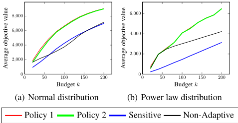
We compute budget allocations over 500 instances by the policies, and compare their objective values by favg(⇡) for a policy ⇡. By preliminary experiments, we verified that 500 instances are enough to compare the average objective values.

Figure 1 indicates the average objective values when the budget k is set to a value in ¶20↪ 40↪ ▷ ▷ ▷ ↪ 200♦. For setting the probabilities qvu of each edge vu, the normal distribution is used in (a), and the power law distribution is used in (b).

Although the theoretical performance guarantee of Policy 2 (in Theorem 4) is inferior to Policy 1 (in Theorem 3), we observe from the experimental results that performances of Policies 1 and 2 are almost same in all instances. Recall that Policy 2 always outputs a feasible allocation whereas Policies 1 does not. Moreover, they are clearly superior to the other two algorithms. In the normal distribution instances, the nonadaptive algorithm is sometimes worse even than the sensitive algorithm. In the power law distribution instances, the nonadaptive algorithm outperforms the sensitive algorithm, but it is clearly worse than Policies 1 and 2.

5.2 General influence model

Adaptive submodularity over an integer lattice is a useful notion, and it has numerous applications other than the budget allocation in the bipartite influence model. Taking advantage of this feature, we extend the budget allocation problem from the bipartite influence model to another influence model defined over general directed graphs. This general influence model can be captured by an adaptive monotone submodular function over an integer lattice, and hence all algorithmic results proposed in this paper can be applied to it. Here, we report empirical performance of the adaptive strategies and the non-adaptive (1 - 1◁e)-approximation algorithm in this general influence model.

We do not describe the detail of the model due to the space limitation. The non-adaptive setting of this model is obtained by introducing multiple influence levels into the independence cascade model studied by Kempe et al. [2003] in a context of influence maximization. We note that a similar attempt can be found in Demaine et al. [2014], but our model is different from theirs. Alon et al. [2012] also mentioned that their bipartite influence model can be naturally extended to general graphs, but they do not seem to consider the multiple influence levels on all nodes.

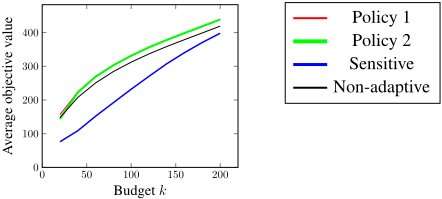
For the experiments, we prepared a graph that represents user-user following information in Twitter [KONECT, 2014]. Each node represents a user, and an arc from a node i to another node j represents that the user corresponding to i is followed by the user corresponding to j. The graph consists of 23370 nodes and 33101 arcs. In this graph, we choose 500 nodes that have largest out-degrees, and consider allocating budgets to these nodes. The parameters in the instances are set as follows: b(v) = 15 for all chosen nodes v, and the objective of the problem is defined as the maximization of the number of nodes influenced at least once. Budget k is set to a value in ¶20↪ 40↪ ▷ ▷ ▷ ↪ 200♦, and the objective values are averaged over 500 instances for each k.

Figure 2 shows the results. Performance of Policies 1 and 2 are nearly equal, the non-adaptive policy is behind them, and the sensitive policy is clearly worse than the others.

6 Conclusion

In this paper, we analyzed adaptive greedy policies for the budget allocation problem. Our contributions are based on the new concept of the adaptive submodularity; we extended the adaptive submodularity defined for the set functions to the functions over integer lattices. We believe that this new concept has other applications than the budget allocation problem. Indeed, we have already studied its applications to data summarization and sensor management. We will report them in the full version of the present paper.