
Nonlinear Hybrid Planning with Deep Net Learned Transition Models and Mixed-Integer Linear Programming
Proceedings of the Twenty-Sixth International Joint Conference on Artificial Intelligence. Main track. Pages 750-756.
https://doi.org/10.24963/ijcai.2017/104
Keywords
- Machine Learning: Deep Learning
- Constraints and Satisfiability: Modeling/Formulation
- Planning and Scheduling: Planning and Scheduling
- Combinatorial & Heuristic Search: Combinatorial search/optimisation
Abstract
In many real-world hybrid (mixed discrete continuous) planning problems such as Reservoir Control, Heating, Ventilation and Air Conditioning (HVAC), and Navigation, it is difficult to obtain a model of the complex nonlinear dynamics that govern state evolution. However, the ubiquity of modern sensors allow us to collect large quantities of data from each of these complex systems and build accurate, nonlinear deep network models of their state transitions. But there remains one major problem for the task of control -- how can we plan with deep network learned transition models without resorting to Monte Carlo Tree Search and other black-box transition model techniques that ignore model structure and do not easily extend to mixed discrete and continuous domains? In this paper, we make the critical observation that the popular Rectified Linear Unit (ReLU) transfer function for deep networks not only allows accurate nonlinear deep net model learning, but also permits a direct compilation of the deep network transition model to a Mixed-Integer Linear Program (MILP) encoding in a planner we call Hybrid Deep MILP Planning (HD-MILP-PLAN). We identify deep net specific optimizations and a simple sparsification method for HD-MILP-PLAN that improve performance over a naive encoding, and show that we are able to plan optimally with respect to the learned deep network.
- [Abadi et al., 2015] Martín Abadi, Ashish Agarwal, Paul Barham, Eugene Brevdo, Zhifeng Chen, Craig Citro, Greg S. Corrado, Andy Davis, Jeffrey Dean, Matthieu Devin, Sanjay Ghemawat, Ian Goodfellow, Andrew Harp, Geoffrey Irving, Michael Isard, Yangqing Jia, Rafal Joze- fowicz, Lukasz Kaiser, Manjunath Kudlur, Josh Leven- berg, Dan Mané, Rajat Monga, Sherry Moore, Derek Mur- ray, Chris Olah, Mike Schuster, Jonathon Shlens, Benoit Steiner, Ilya Sutskever, Kunal Talwar, Paul Tucker, Vin- cent Vanhoucke, Vijay Vasudevan, Fernanda Viégas, Oriol Vinyals, Pete Warden, Martin Wattenberg, Martin Wicke, Yuan Yu, and Xiaoqiang Zheng. TensorFlow: Large-scale machine learning on heterogeneous systems, 2015.
- [Agarwal et al., 2010] Yuvraj Agarwal, Bharathan Balaji, Rajesh Gupta, Jacob Lyles, Michael Wei, and Thomas Weng. Occupancy-driven energy management for smart building automation. In ACM Workshop on Embedded Sensing Systems for Energy-Efficiency in Building, pages 1-6, 2010.
- [Bryce et al., 2015] Daniel Bryce, Sicun Gao, David Musliner, and Robert Goldman. SMT-based nonlinear PDDL+ planning. In 29th AAAI, pages 3247-3253, 2015.
- [Cashmore et al., 2016] Michael Cashmore, Maria Fox, Derek Long, and Daniele Magazzeni. A compilation of the full PDDL+ language into SMT. In ICAPS, pages 79- 87, 2016.
- [Coles et al., 2013] Amanda J. Coles, Andrew Coles, Maria Fox, and Derek Long. A hybrid LP-RPG heuristic for modelling numeric resource flows in planning. JAIR, pages 343-412, 2013.
- [Coulom, 2006] Rémi Coulom. Efficient selectivity and backup operators in monte-carlo tree search. In Interna- tional Conference on Computers and Games, pages 72-83. Springer Berlin Heidelberg, 2006.
- [D'Andreagiovanni and Gleixner, 2016] Fabio D'Andreagiovanni and Ambros M. Gleixner. Towards an Accurate Solution of Wireless Network Design Problems, pages 135-147. Springer International Publishing, 2016.
- [Faulwasser and Findeisen, 2009] Timm Faulwasser and Rolf Findeisen. Nonlinear Model Predictive Path- Following Control. In Nonlinear Model Predictive Control -Towards New Challenging Applications, pages 335-343. Springer, Berlin, Heidelberg, 2009.
- [Fox and Long, 2006] Maria Fox and Derek Long. Mod- elling mixed discrete-continuous domains for planning. JAIR, pages 235-297, 2006.
- [Huang et al., 2016] Gao Huang, Zhuang Liu, and Kilian Q Weinberger. Densely connected convolutional networks. arXiv preprint arXiv:1608.06993, 2016.
- [Ivankovic et al., 2014] Franc Ivankovic, Patrik Haslum, Sylvie Thiebaux, Vikas Shivashankar, and Dana Nau. Op- timal planning with global numerical state constraints. In ICAPS, pages 145-153, 2014.
- [Keller and Helmert, 2013] Thomas Keller and Malte Helmert. Trial-based heuristic tree search for finite horizon MDPs. In ICAPS, pages 135-143, 2013.
- [Kocsis and Szepesvári, 2006] Levente Kocsis and Csaba Szepesvári. Bandit based Monte-Carlo planning. In ECML, pages 282-293, 2006.
- [Löhr et al., 2012] Johannes Löhr, Patrick Eyerich, Thomas Keller, and Bernhard Nebel. A planning based framework for controlling hybrid systems. In ICAPS, pages 164-171, 2012.
- [Mnih et al., 2013] Volodymyr Mnih, Koray Kavukcuoglu, David Silver, Alex Graves, Ioannis Antonoglou, Daan Wierstra, and Martin Riedmiller. Playing atari with deep reinforcement learning. In NIPS Deep Learning Work- shop. 2013.
- [Nair and Hinton, 2010] Vinod Nair and Geoffrey E. Hinton. Rectified linear units improve restricted boltzmann ma- chines. In ICML, pages 807-814, 2010.
- [Penna et al., 2009] Giuseppe Della Penna, Daniele Maga- zzeni, Fabio Mercorio, and Benedetto Intrigila. UPMur- phi: A tool for universal planning on PDDL+ problems. In ICAPS, pages 106-113, 2009.
- [Piotrowski et al., 2016] Wiktor Mateusz Piotrowski, Maria Fox, Derek Long, Daniele Magazzeni, and Fabio Merco- rio. Heuristic planning for hybrid systems. In AAAI, pages 4254-4255, 2016.
- [Scala et al., 2016a] Enrico Scala, Patrik Haslum, Sylvie Thiébaux, and Miquel Ramírez. Interval-based relaxation for general numeric planning. In ECAI, pages 655-663, 2016.
- [Scala et al., 2016b] Enrico Scala, Miquel Ramirez, Patrik Haslum, and Sylvie Thiebaux. Numeric planning with dis- junctive global constraints via SMT. In ICAPS, pages 276- 284, 2016.
- [Silver et al., 2016] David Silver, Aja Huang, Christopher J. Maddison, Arthur Guez, Laurent Sifre, George van den Driessche, Julian Schrittwieser, Ioannis Antonoglou, Veda Panneershelvam, Marc Lanctot, Sander Dieleman, Do- minik Grewe, John Nham, Nal Kalchbrenner, Ilya Sutskever, Timothy Lillicrap, Madeleine Leach, Koray Kavukcuoglu, Thore Graepel, and Demis Hassabis. Mas- tering the game of go with deep neural networks and tree search. Nature, pages 484-503, 2016.
- [Sutton and Barto, 1998] Richard S. Sutton and Andrew G. Barto. Introduction to Reinforcement Learning. MIT Press, 1st edition, 1998.
- [Szepesvári, 2010] Csaba Szepesvári. Algorithms for Rein- forcement Learning. Morgan & Claypool, 2010.
- [Weinstein and Littman, 2012] Ari Weinstein and Michael L. Littman. Bandit-based planning and learning in continuous-action markov decision processes. In ICAPS, 2012.
- [Yeh, 1985] William G Yeh. Reservoir management and operations models: A state-of-the-art review. Water Re- sources research, 21,12:17971818, 1985.
References were extracted automatically from the PDF and may contain errors.
Full text extracted automatically from the PDF; figures, tables and equations may differ. The PDF is the version of record.
1 Introduction
In many real-world hybrid (mixed discrete continuous) planning problems such as Reservoir Control [Yeh, 1985], Heating, Ventilation and Air Conditioning (HVAC) [Agarwal et al., 2010], and Navigation [Faulwasser and Findeisen, 2009], it is difficult to obtain a model of the complex nonlinear dynamics that govern state evolution. For example, in Reservoir Control, evaporation and other sources of water loss are a complex function of volume, bathymetry, and environmental conditions; in HVAC domains, thermal conductance between walls and convection properties of rooms are nearly impossible to derive from architectural layouts; and in Navigation problems, nonlinear interactions between surfaces and traction devices make it hard to accurately predict odometry.
A natural answer to these modeling difficulties is to instead learn the transition model from sampled data; fortunately, the presence of vast sensor networks often make such data inexpensive and abundant. While learning nonlinear models with a priori unknown model structure can be very difficult in practice, recent progress in Deep Learning and the availability of off-the-shelf tools such as TensorFlow [Abadi et al., 2015] make it possible to learn highly accurate nonlinear deep neural networks with little prior knowledge of model structure as we will demonstrate experimentally in this paper.
However, the modeling of a nonlinear transition model as a deep neural network poses non-trivial difficulties for the optimal control task. Existing hybrid planners either are not compatible with nonlinear deep net transition models and continuous action input [Penna et al., 2009; L¨ohr et al., 2012; Coles et al., 2013; Ivankovic et al., 2014; Piotrowski et al., 2016; Scala et al., 2016a], or only optimize goal-oriented objectives [Bryce et al., 2015; Scala et al., 2016b; Cashmore et al., 2016]. Monte Carlo Tree Search (MCTS) methods [Coulom, 2006; Kocsis and Szepesv´ari, 2006; Keller and Helmert, 2013] including AlphaGo [Silver et al., 2016] that could exploit a deep net learned black box model of transition dynamics do not inherently work with continuous action spaces due to the infinite branching factor. While MCTS with continuous action extensions such as HOOT [Weinstein and Littman, 2012] have been proposed, their continuous partitioning methods do not scale to high-dimensional continuous action spaces. Finally, offline model-free reinforcement learning with function approximation [Sutton and Barto, 1998; Szepesv´ari, 2010] and deep extensions [Mnih et al., 2013] do not directly apply to domains with high-dimensional continuous action spaces. That is, offline learning methods like Q-learning require action maximization for every update, but in high-dimensional continuous action spaces such nonlinear function maximization is non-convex and computationally intractable at the scale of millions or billions of updates.
Despite these limitations of existing methods, all is not lost. First, we remark that our deep net is not a black-box but rather a gray-box; while the learned parameters often lack human interpretability, there is still a uniform layered symbolic structure in the deep models. Second, we make the critical observation that the popular Rectified Linear Unit (ReLU) [Nair and Hinton, 2010] transfer function for deep networks allows accurate nonlinear deep net model learning and permits a direct compilation to a Mixed-Integer Linear Program (MILP) encoding. Given other components such as a humanspecified objective function and a horizon, this permits direct optimization in a method we call Hybrid Deep MILP Planning (HD-MILP-PLAN). We evaluate HD-MILP-PLAN on Reservoir Control, HVAC and Navigation domains, and identify a number of domain-independent strengthening constraints and a simple sparsification approach that improve performance over a na¨ıve encoding. Ultimately our results show deep learning with MILP-based control is a promising new direction for nonlinear hybrid planning problems.
2 Preliminaries
Before we discuss deep net transition learning, we review the hybrid nonlinear planning problem motivating this work.
2.1 Hybrid Planning with Nonlinear Transitions
A hybrid planning problem is a tuple Π = 〈S, A, C, T, I, Q〉 where S = {Sd , Sc } is a mixed set of state variables (states) with discrete Sd and continuous Sc domains, A = {Ad , Ac } is a mixed set of action variables (actions) with discrete Ad and continuous Ac domains, C : S × A → {true, false} is a function that returns true if action a ∈ A and state s ∈ S pair satisfies linear constraints that represent action preconditions, T : S×A → S denotes the transition function between time steps t and t+1 (time is uniformly discretized) such that T (st , at ) = st+1 if C(st , at ) = true and is undefined otherwise. Finally, I is the initial state and Q : S×A → R denotes the state-action reward function. Given a planning horizon H, an optimal solution to Π is a plan that maximizes the total reward function over horizon H such that ∑Ht=1 Q(st+1 , at ).
In many real-world problems, it is difficult to model the exact dynamics of the complex nonlinear transition function T that governs the evolution of states S over the horizon H. Therefore in this paper, we do not assume a-priori knowledge on T, but rather we learn it from data. We limit our model knowledge to our reward function Q, horizon H and simple action-precondition function C that specifies whether actions a are applicable in state s at time t, or not, e.g., the outflow from a reservoir must not exceed the present water level.
2.2 Deep Net Transition Learning
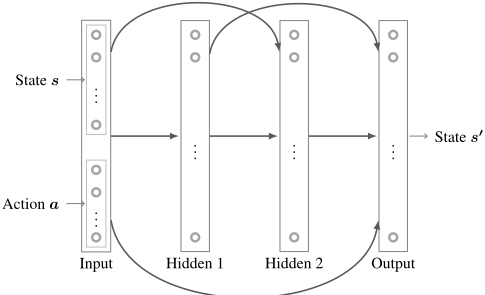
We model our state transition function as a deep neural network as shown in Figure 1. This deep neural network is a layered, acyclic, directed network structure with linear transforms of the outputs from one layer to the input of the next layer and potentially nonlinear transfer functions at each layer. Specifically, the output layer uses a linear (identity) transfer function while all hidden layers use nonlinear (piecewise linear) Rectified Linear Units (ReLUs) [Nair and Hinton, 2010] of the form relu(x) = max(x, 0). In comparison to the other activation functions, such as sigmoid and hyperbolic tangent, ReLUs can be trained efficiently and permit direct compilation to a set of linear constraints.
We use a densely-connected network [Huang et al., 2016] as shown in Figure 1, which in comparison to a standard fully connected network allows direct connections of each layer to the output. This can be advantageous when a transition function has differing levels of nonlinearity - linear transitions can pass directly from the input to the output layer, while nonlinear transitions may pass through one or more of the hidden layers. Given a deep neural net configuration with L hidden layers, state vectors S, S′ and an action vector A from data D={(S1,A1, S1 ′ ), . . . , (Sn,An, Sn′ )} and a hyperparameter λ, the optimal weights Wl for all layers {1, . . . ,L} can be found by solving the following optimization problem:
subject to
The objective minimizes squared reconstruction error of transitions in the data plus a regularizer. Constraints (1) and (2) define the ReLU vector of Zl for each layer l∈{1,...,L-1} and outputs ˜ S′, where || denotes the concatenation operation.
3 Hybrid DeepMILP Planning
Hybrid Deep MILP Planning (HD-MILP-PLAN) is a twostage framework for learning and optimizing nonlinear hybrid planning problems. The first stage of HD-MILP-PLAN learns the unknown transition function T using a densely-connected deep neural network defined above. The learned transition function ˜ T is used to construct the model ˜Π=〈S,A,C, ˜ T ,I ,Q〉, which is provided to our MILP-based hybrid planner as a parameter. Given a planning horizon H, the second stage of HD-MILP-PLAN finds an optimal plan to the learned-model ˜Π using a Mixed Integer Linear Program (MILP). HD-MILPPLAN operates as an online planner where actions are optimized over the remaining planning horizon in response to sequential state observations from the environment.
We now describe an initial MILP encoding of HD-MILPPLAN. Then, we strengthen the linear relaxation of our na¨ıve MILP encoding and sparsify it for solver efficiency.
3.1 Na¨ıve MILP-based Hybrid Planner
We begin with all notation necessary for the specification:
Parameters
- VI(s) is the value of the initial state s∈S.
- R is the set of ReLUs in the neural network.
- B is the set of bias units in the neural network.
- O is the set of output units in the neural network.
- E is the set of synapsis in the neural network.
- W is the set of weights in the neural network.
- A(f) is the set of actions connected to unit f∈R∪O.
- S(f) is the set of states connected to unit f∈R∪O.
- U(f) is the set of units connected to f∈R∪O.
- O(s) specifies the output unit that predicts state s∈S.
- M is a large constant used in the big-M constraints.
Decision variables
- Xat denotes the value assignment to action a∈A from its domain at time t. The domain of Xat can be either discrete or continuous.
- Yst denotes the value of state s∈S at time t. The domain of Yst can be either discrete or continuous.
- Pft denotes the output of unit f∈R at time t.
- P b ft=1 if rectified linear unit f∈R is activated at time t, 0 otherwise (i.e., P b ft is a boolean variable).
Na¨ıve MILP encoding
Next we define the MILP formulation of our planning optimization problem that encodes the learned transition model.
subject to
for all time steps t=1,...,H except Constraint (1)
In the above MILP, the objective maximizes the sum of rewards over a given horizon H. Constraint (1) connects input units of the neural network to the initial state of the planning problem at time t=1. Constraint (2) sets all neurons that represent biases equal to 1. Constraint (3) ensures that a ReLU f∈R is activated if the total weighted input flow into f is positive. Constraints (4)-(5) together ensure that if a ReLU f∈R is active, the outflow from f is equal to the total weighted input flow. Constraint (6) connects two states St and St+1 at two consecutive times t and t+1 for all t=1,...,H. Constraint (7) ensures that action preconditions are satisfied at every time t.
Note that Constraints (3)-(5) sufficiently encode the piecewise linear activation function of the ReLUs. However, the positive unbounded nature of the ReLUs leads to a poor linear relaxation of the big-M constraints, that is, when all boolean variables (superscripted with b) are relaxed to continuous [0,1] in Constraints (3)-(4); this can significantly hinder the overall performance of standard branch and bound MILP solvers that rely on the linear relaxation of the MILP for heuristic guidance. Next, we strengthen our na¨ıve MILP encoding with the addition of auxiliary decision variables and linear constraints with the same solution as the na¨ıve MILP encoding, but a tighter LP relaxation that we subsequently observe to significantly improve MILP optimization time.
Strengthened MILP-based hybrid planner
In our na¨ıve MILP encoding, Constraints (4)-(6) encode the piecewise linear activation function, relu(x)=max(x,0), using the big-M constraints for each ReLU f∈R. We strengthen the linear relaxation of Constraints (5)-(6) by first separating the input x into its positive x+ and negative x- components. Using these auxiliary variables, we augment our na¨ıve MILP encoding with an additional linear inequality in the form of x+≥relu(x). This inequality is valid since the constraints x= x+-x- and relu(x)=max(x,0)≤max(x+,0)=x+ hold for all x+,x-≥0. The additional decision variables required to implement our strengthened MILP are as follows:
- X+ at and Xat denote the positive and negative value assignments to action a∈A at time t, respectively.
- Y + st and Y - st denote the positive and negative the values of state s∈S at time t, respectively.
- Xbat=1 if Xat is positive at time t, 0 otherwise.
- Y b st=1 if Yst is positive at time t, 0 otherwise.
The additional constraints in the strengthened MILP are then
for all actions a∈A where La<0, time steps t=0,...,H
for all states s∈S where Ls<0, time steps t=1,...,H+1
Here, the pairs 〈La,Ua〉 and 〈Ls,Us〉 denote the lower and upper bounds on the domains of action a∈A and state s∈S decision variables Xat, Yst, respectively. Note that if either of the upper bounds Ua or Us are negative, the planning problem Π must be transformed into an equivalent problem Π′ where upper bounds Ua,Us on every action a∈A and state s∈S are non-negative. Given Constraints (8)-(17), Constraint (18) implements our strengthening constraint which provides a valid upper bound on each ReLU f∈R.
for all ReLU g∈R, time steps t=0,...,H
Network sparsification
In both na¨ıve and strengthened MILP encodings, Constraints (4)-(6) are linear expressions often with very small weights that do not contribute a significant amount to the output of a unit. Computationally, MILP formulations with very small constraint coefficients can be challenging to solve for stateof-the-art solvers [D'Andreagiovanni and Gleixner, 2016]. To tackle this issue, we implement a sparsification approach to remove connections to and from ReLUs with very small weights. Given a sparsification parameter 0≤β≤1, we set wij=0 if |wij| is less than the ⌊β×|W|⌋-th smallest element from the set of absolute weight values.
4 Experimental Results
In this section, we introduce our three hybrid nonlinear benchmark domains and then validate our HD-MILP-PLAN framework with respect to the following experiments. First, we evaluate the transition learning performance of ReLUbased deep networks in each domain. Then, we evaluate MILP planning efficacy based on the learned model by comparing it to strong baseline manually coded policies. As noted in the Introduction, MCTS and model-free reinforcement learning are not applicable as baselines given our multi-dimensional concurrent continuous action spaces. Since learning is the only method of estimating an arbitrary nonlinear transition function from data, it is an open research question how best to compile a deep network to the input of PDDL+ [Fox and Long, 2006] hybrid planners. 1 Finally, we compare the efficiency of the na¨ıve and strengthened MILP encodings, and measure the computational gains when using sparsified transitions.
4.1 Illustrative Domains
Reservoir Control has a single state lr∈R for each reservoir, which denotes the water level of the reservoir r and a corresponding action for each r to permit a flow fr∈[0,rmax] from reservoir r (with maximum allowable flow rmax) to the next downstream reservoir. The transition is nonlinear function due to the evaporation er from each reservoir r, which is defined by the formula
1 We see three ways of encoding a deep net in PDDL+: the network can either be flattened into a single piecewise function which will blow up exponentially in the network size, or the output of ReLUs could be encoded as derived predicates for planners that support them, or each ReLU could be modeled as an exogenous event. It is not clear how modern PDDL+ planners would perform under any of the above encodings and we will investigate this in future work.
and the water level transition function is
where frup ranges over all upstream reservoirs of r. The reward function minimizes the total absolute deviation from a desired water level, plus a constant penalty for having water level outside of a safe range (close to empty or overflowing), which is defined for each time step t by the formula
where mr and nr define the upper and and lower desired ranges for each reservoir r. We report the results on instances with 3 and 4 reservoirs over planning horizons H=10,20.
Heating, Ventilation and Air Conditioning [Agarwal et al., 2010] has a state variable pr∈R denoting the temperature of each room r and an action br∈[0,bmax] for sending heated air to each room r (with maximum allowable volume bmax) via vent actuation. The bilinear transition function is then
where Cr is the heat capacity of rooms, r′ represents an adjacency predicate with respect to room r and Rrr′ represents a thermal conductance between rooms. The reward function minimizes the total absolute deviation from a desired temperature for all rooms plus a linear penalty for having temperatures outside of a range plus a linear penalty for heating air with cost k, and is defined for each time step t by the formula
We report the results on instances with 3 and 6 rooms over planning horizons H=10,20.
Navigation is designed to test learning of a highly nonlinear transition function and has a single state for the 2D location of an agent pt+1 and a 2D action intended nominally to move the agent ∆p. The new location pt+1 is a nonlinear function of the current location pt due to higher slippage in the center of the domain where the transition function is
where ∆dp is the Euclidean distance from p to the center of the domain. The reward function minimizes the total Manhattan distance from the goal location, which is defined for each time step t by the formula
| Domain | Linear | 1 Hidden | 2 Hidden |
| Reservoir | 46500000 ±487000 | 343000 ±7210 | 653000 ±85700 |
| HVAC | 710±2.3 | 520±54 | 75200±7100 |
| Navigation | 30440±9.8 | 9420±29 | 1940±50 |
where gd defines the goal location for dimension d. We report the results on instances with maze sizes 8-by-8 and 10-by-10 over planning horizons H=8,10.
4.2 Transition Learning Performance
In Table 1, we show the mean squared error of learning for different configurations of the deep net on each domain. The policy generating the sample data was a simple stochastic exploration policy and the deep nets were tested on a held-out set of sample data. The sampled data was generated in the sizes of 105 data points for all domains and treated as independent and identically distributed. After random permutation, the sampled data was split into training and test sets with 4 to 1 ratio. Dense deep networks [Huang et al., 2016] strictly dominated non-dense networks so we only report dense network results. Overall, we see that Reservoir and HVAC could be accurately learned with one layer (an additional layer did not help) while Navigation benefited from having two layers owing to the complexity of its transition. The lowest MSE deep net was used as the deep net model for each domain in subsequent planning experiments.
4.3 Planning Performance
In this section, we investigate the effectiveness of using a MILP-based hybrid planner to optimize a learned-model ˜Π. We ran our experiments on a Linux system with two 20core CPUs, 256GB Memory. We optimized our MILP encodings using IBM ILOG CPLEX 12.6.3 with 32 threads and a 1-hour total time limit per problem instance. We connected HD-MILP-PLAN with the domain simulator and interactively solved 12 problem instances where the instances were generated from three domains with two different problem sizes and two different horizon lengths. For the sparsification approach, we have picked the parameter to be β=0.15.
Comparative performance per domain
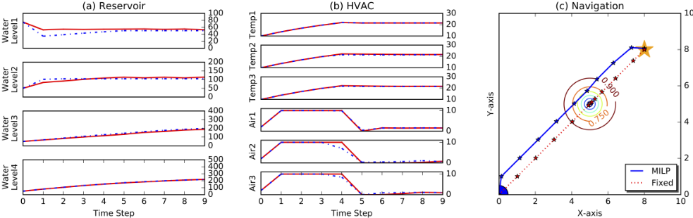
In Figure 2 (a), we compare HD-MILP-PLAN with two network settings to a rule-based local Reservoir planner, which measures the water level in reservoirs, and sets outflows to release water above a pre-specified median level of reservoir capacity. In this domain, we observe an average of 15% increase in the total reward obtained by the plans generated by HD-MILP-PLAN with a non-sparse network in comparison to that of the rule-based local Reservoir planner. Similarly, we find that HD-MILP-PLAN with a sparsified network outperforms the rule-based local Reservoir planner by an average of 8%. In Figure 3 (a), we see in the two subplots that HDMILP-PLAN with a non-sparse network was able to use its model of evaporation to maintain a more stable water level than the threshold-triggered manual policy.
In Figure 2 (b), we compare HD-MILP-PLAN with both network settings to a rule-based local HVAC policy, which turns on the air conditioner anytime the room temperature is below the median value of a given range of comfortable temperatures [20,25], and turns off otherwise. We observe that the plans generated by HD-MILP-PLAN under both network settings are almost identical to that of the locally optimal HVAC policy. However, in Figure 3 (b), we observe that HVAC is able to exploit its model of thermal conductivity to stop heating rooms (bottom two subplots, dashed blue line below red line) before the manual policy cuts off.
Figure 2 (c) compares HD-MILP-PLAN under both network settings to a greedy search policy, which uses a Manhattan distance-to-goal function to guide the agent towards the direction of the goal (cf. Figure 3 (c)). The pairwise comparison of the total rewards obtained for each problem instance per plan shows that HD-MILP-PLAN with both network settings can outperform the manual policy upto 42%, as observed in the problem instance Navigation,10,8 in Figure 2 (c). The investigation of the actual plans, as visualized by Figure 3 (c), shows that the local policy ignores the nonlinear region in the middle, and tries to reach the goal directly. In contrast, HD-MILP-PLAN under both network settings can find plans that move around the nonlinearity, due to its ability to model the nonlinearity and find a plan that is optimal with respect to the learned model over the complete horizon H.
Overall we observe that in 8 out of 12 problem instances, the solution quality of the plans generated by HD-MILPPLAN with both network settings are significantly better than the total reward obtained by the plans generated by the respective domain-specific human-designed policies.
Comparative performance per MILP encoding
In Figures 4 (a)-(c), the black and blue bars give a run time comparison of our na¨ıve MILP encoding to its strengthened version given the time-limit of 1 hour. Figures 4 (a)-(c) show moderate, none and significant run time improvement for the strengthened encoding over our na¨ıve MILP encoding.
Comparative performance per network setting
The pairwise comparison of HD-MILP-PLAN with a sparsified network over a non-sparse network shows that the planning qualities were identical in HVAC and Navigation domains and less than 5% worse in the Reservoir domain. In 11 out of 12 problem instances, our sparsification approach improved the run time performance of HD-MILP-PLAN up to 80% (see Navigation,10,8 in Figures 4 (c)).
5 Conclusion
In this paper, we have tackled the question of how we can plan with expressive and accurate deep network learned transition models that are not amenable to existing solution techniques. We leveraged the insight that ReLU based deep networks offer strong learning performance and permit a direct compilation of the deep network transition model to a Mixed-Integer Linear Program (MILP) encoding in a planner we called Hybrid Deep MILP Planning (HD-MILP-PLAN). To enhance planning efficiency, we have strengthened the linear relaxation of the na¨ıve MILP encoding and simplified our deep networks through sparsification.


We evaluated run time performance and solution quality of the plans generated by HD-MILP-PLAN under both network settings and MILP encodings over 12 problem instances from three planning domains. We have shown that HD-MILPPLAN can accurately learn unknown transition functions and find optimal plans with respect to the learned models. We have shown that the plans generated by HD-MILP-PLAN yield better solution qualities compared to strong domainspecific human-designed policies. Finally we have shown that both our strengthening constraints and network sparsification improved the run time performance of HD-MILP-PLAN. In conclusion, HD-MILP-PLAN represents a new class of datadriven planning methods that can provide bounded optimality guarantees with respect to deep network learned transition models and offers strong empirical performance over a variety of high-dimensional nonlinear hybrid planning domains.
@inproceedings{ijcai2017p104,
  title     = {Nonlinear Hybrid Planning with Deep Net Learned Transition Models and Mixed-Integer Linear Programming},
  author    = {Say, Buser and Wu, Ga and Zhou, Yu Qing and Sanner, Scott},
  booktitle = {Proceedings of the Twenty-Sixth International Joint Conference on
               Artificial Intelligence, {IJCAI-17}},
  publisher = {International Joint Conferences on Artificial Intelligence Organization},
  editor    = {Carles Sierra},
  pages     = {750--756},
  year      = {2017},
  month     = {8},
  note      = {Main track},
  doi       = {10.24963/ijcai.2017/104},
  url       = {https://doi.org/10.24963/ijcai.2017/104},
}
TY - CPAPER TI - Nonlinear Hybrid Planning with Deep Net Learned Transition Models and Mixed-Integer Linear Programming AU - Say, Buser AU - Wu, Ga AU - Zhou, Yu Qing AU - Sanner, Scott T2 - Proceedings of the Twenty-Sixth International Joint Conference on Artificial Intelligence, IJCAI-17 PB - International Joint Conferences on Artificial Intelligence Organization PY - 2017 SP - 750 EP - 756 DO - 10.24963/ijcai.2017/104 UR - https://doi.org/10.24963/ijcai.2017/104 ER -Copied
Machine-readable versions of this paper, for tools and AI agents:





