
Search and Learn: On Dead-End Detectors, the Traps they Set, and Trap Learning
Proceedings of the Twenty-Sixth International Joint Conference on Artificial Intelligence. Main track. Pages 4398-4404.
https://doi.org/10.24963/ijcai.2017/614
Keywords
- Combinatorial & Heuristic Search: Heuristic Search
- Planning and Scheduling: Search in Planning and Scheduling
- Planning and Scheduling: Planning Algorithms
Abstract
A key technique for proving unsolvability in classical planning are dead-end detectors \Delta: effectively testable criteria sufficient for unsolvability, pruning (some) unsolvable states during search. Related to this, a recent proposal is the identification of traps prior to search, compact representations of non-goal state sets T that cannot be escaped. Here, we create new synergy across these ideas. We define a generalized concept of traps, relative to a given dead-end detector \Delta, where T can be escaped, but only into dead-end states detected by \Delta. We show how to learn compact representations of such T during search, extending the reach of \Delta. Our experiments show that this can be quite beneficial. It improves coverage for many unsolvable benchmark planning domains and dead-end detectors \Delta, in particular on resource-constrained domains where it outperforms the state of the art.
- [Bacchus, 2001] Fahiem Bacchus. The AIPS'00 planning competi- tion. AI Magazine, 22(3):47-56, 2001.
- [Bäckström et al., 2013] Christer Bäckström, Peter Jonsson, and Simon Ståhlberg. Fast detection of unsolvable planning instances using local consistency. Proc. SOCS'13, 29-37.
- [Blum and Furst, 1997] Avrim L. Blum and Merrick L. Furst. Fast planning through planning graph analysis. AI, 90(1-2):279-298, 1997.
- [Bradley, 2011] Aaron R. Bradley. Sat-based model checking with- out unrolling. Proc. VMCAI'11, 70-87.
- [Coles et al., 2012] Amanda Jane Coles, Andrew Coles, Angel García Olaya, Sergio Jiménez, Carlos Linares López, Scott San- ner, and Sungwook Yoon. A survey of the seventh international planning competition. AI Magazine, 33(1), 2012.
- [Coles et al., 2013] Amanda Jane Coles, Andrew Coles, Maria Fox, and Derek Long. A hybrid LP-RPG heuristic for modelling nu- meric resource flows in planning. JAIR, 46:343-412, 2013.
- [Domshlak and Mirkis, 2015] Carmel Domshlak and Vitaly Mirkis. Deterministic oversubscription planning as heuristic search: Ab- stractions and reformulations. JAIR, 52:97-169, 2015.
- [Domshlak et al., 2015] Carmel Domshlak, Jörg Hoffmann, and Michael Katz. Red-black planning: A new systematic approach to partial delete relaxation. AI, 221:73-114, 2015.
- [Edelkamp et al., 2004] Stefan Edelkamp, Alberto Lluch-Lafuente, and Stefan Leue. Directed explicit-state model checking in the validation of communication protocols. International Journal on Software Tools for Technology Transfer, 5(2-3):247-267, 2004.
- [Edelkamp, 2001] Stefan Edelkamp. Planning with pattern databases. Proc. ECP'01, 13-24.
- [Gerevini et al., 2009] Alfonso Gerevini, Patrik Haslum, Derek Long, Alessandro Saetti, and Yannis Dimopoulos. Deterministic planning in the fifth international planning competition: PDDL3 and experimental evaluation of the planners. AI, 173(5-6):619- 668, 2009.
- [Gnad et al., 2016] Daniel Gnad, Marcel Steinmetz, and Jörg Hoff- mann. Django: Unchaining the power of red-black planning. UIPC 2016 planner abstracts, 19-23.
- [Haslum and Geffner, 2000] Patrik Haslum and Hector Geffner. Admissible heuristics for optimal planning. Proc. AIPS'00, 140- 149.
- [Helmert et al., 2014] Malte Helmert, Patrik Haslum, Jörg Hoff- mann, and Raz Nissim. Merge & shrink abstraction: A method for generating lower bounds in factored state spaces. JACM, 61(3), 2014.
- [Helmert, 2006] Malte Helmert. The Fast Downward planning sys- tem. JAIR, 26:191-246, 2006.
- [Hoffmann and Edelkamp, 2005] Jörg Hoffmann and Stefan Edelkamp. The deterministic part of ipc-4: An overview. JAIR, 24:519-579, 2005.
- [Hoffmann et al., 2014] Jörg Hoffmann, Peter Kissmann, and Álvaro Torralba. "Distance"? Who Cares? Tailoring merge-and- shrink heuristics to detect unsolvability. Proc. ECAI'14.
- [Kambhampati, 2000] Subbarao Kambhampati. Planning graph as a (dynamic) CSP: Exploiting EBL, DDB and other CSP search techniques in graphplan. JAIR, 12:1-34, 2000.
- [Kolobov et al., 2012] Andrey Kolobov, Mausam, and Daniel S. Weld. Discovering hidden structure in factored MDPs. AI, 189:19-47, 2012.
- [Kupferschmid et al., 2006] Sebastian Kupferschmid, Jörg Hoff- mann, Henning Dierks, and Gerd Behrmann. Adapting an AI planning heuristic for directed model checking. Proc. SPIN 2006, 35-52.
- [Kupferschmid et al., 2008] Sebastian Kupferschmid, Jörg Hoff- mann, and Kim G. Larsen. Fast directed model checking via Russian doll abstraction. Proc. TACAS'08, 203-217.
- [Laborie and Ghallab, 1995] P. Laborie and M. Ghallab. Planning with sharable resource constraints. Proc. IJCAI'95, 1643-1649.
- [Lipovetzky et al., 2016] Nir Lipovetzky, Christian J. Muise, and Hector Geffner. Traps, invariants, and dead-ends. Proc. ICAPS'16, 211-215.
- [Long and Fox, 1999] Derek Long and Maria Fox. Efficient imple- mentation of the plan graph in stan. JAIR, 10:87-115, 1999.
- [Long and Fox, 2003] Derek Long and Maria Fox. The 3rd inter- national planning competition: Results and analysis. JAIR, 20:1- 59, 2003.
- [Nakhost et al., 2012] Hootan Nakhost, Jörg Hoffmann, and Martin Müller. Resource-constrained planning: A Monte Carlo random walk approach. Proc. ICAPS'12, 181-189.
- [Pommerening and Seipp, 2016] Florian Pommerening and Jendrik Seipp. Fast downward dead-end pattern database. UIPC 2016 planner abstracts, 2-2.
- [Pommerening et al., 2014] Florian Pommerening, Gabriele Röger, Malte Helmert, and Blai Bonet. LP-based heuristics for cost- optimal planning. Proc. ICAPS'14.
- [Pommerening et al., 2015] Florian Pommerening, Malte Helmert, Gabriele Röger, and Jendrik Seipp. From non-negative to general operator cost partitioning. Proc. AAAI'15, 3335-3341.
- [Seipp et al., 2016] Jendrik Seipp, Florian Pommerening, Silvan Sievers, and Martin Wehrle. Fast downward aidos. UIPC 2016 planner abstracts, 28-38.
- [Smith, 2004] David E. Smith. Choosing objectives in over- subscription planning. Proc. ICAPS'04, 393-401.
- [Steinmetz and Hoffmann, 2016a] Marcel Steinmetz and Jörg Hoffmann. Clone: A critical-path driven clause learner. UIPC 2016 planner abstracts, 24-27.
- [Steinmetz and Hoffmann, 2016b] Marcel Steinmetz and Jörg Hoffmann. Towards clause-learning state space search: Learning to recognize dead-ends. Proc. AAAI'16.
- [Steinmetz and Hoffmann, 2017] Marcel Steinmetz and Jörg Hoff- mann. State space search nogood learning: Online refinement of critical-path dead-end detectors in planning. AI, 2017. In press.
- [Suda, 2014] Martin Suda. Property directed reachability for auto- mated planning. JAIR, 50:265-319, 2014.
- [Torralba and Alcázar, 2013] Álvaro Torralba and Vidal Alcázar. Constrained symbolic search: On mutexes, BDD minimization and more. Proc. SOCS'13, 175-183.
- [Torralba et al., 2016] Álvaro Torralba, Jörg Hoffmann, and Peter Kissmann. MS-Unsat and SimulationDominance: Merge-and- shrink and dominance pruning for proving unsolvability. UIPC 2016 planner abstracts, 12-15.
- [Torralba, 2016] Álvaro Torralba. Sympa: Symbolic perimeter ab- stractions for proving unsolvability. UIPC 2016 planner ab- stracts, 8-11.
References were extracted automatically from the PDF and may contain errors.
Full text extracted automatically from the PDF; figures, tables and equations may differ. The PDF is the version of record.
1 Introduction
Classical planning is concerned with the analysis of goal reachability in large state spaces, compactly described in terms of planning tasks specifying a vector of state variables, an initial state, a set of actions, and a goal condition. Planning research has traditionally been concerned with solvable tasks, reflected for example in the benchmarks used in the International Planning Competition (IPC) up to the year 2014 [Bacchus, 2001; Long and Fox, 2003; Hoffmann and Edelkamp, 2005; Gerevini et al., 2009; Coles et al., 2012]. However, proving planning tasks unsolvable is also quite relevant in practice. Unsolvable tasks occur, for example, in oversubscription planning [Smith, 2004; Gerevini et al., 2009; Domshlak and Mirkis, 2015] and in directed model checking [Edelkamp et al., 2004; Kupferschmid et al., 2006; 2008]. Furthermore, even solvable planning tasks often contain unsolvable - dead-end - states, for example when dealing with limited resources [Laborie and Ghallab, 1995; Nakhost et al., 2012; Coles et al., 2013].
Research in classical planning has recently seen a surge of techniques addressing these issues, designing effective techniques for proving unsolvability. After initial works [B¨ackstr¨om et al., 2013; Hoffmann et al., 2014], a wealth of techniques participated in the inaugural Unsolvability International Planning Competition (UIPC'16) (e. g., [Torralba and Alc´azar, 2013; Domshlak et al., 2015; Torralba et al., 2016; Pommerening and Seipp, 2016; Seipp et al., 2016; Steinmetz and Hoffmann, 2016a; Torralba, 2016; Gnad et al., 2016]). One major strand of these works designs what we will refer to as dead-end detectors ∆: effectively testable criteria sufficient for unsolvability, designed to be called on every state during search, serving to prune those dead-end states detected. Such ∆ were designed based on suitable variants of heuristic functions, namely pattern databases [Edelkamp, 2001], merge-and-shrink heuristics [Helmert et al., 2014; Hoffmann et al., 2014], potential heuristics [Pommerening et al., 2015], and critical-path heuristics [Haslum and Geffner, 2000; Steinmetz and Hoffmann, 2016b; 2017]. These detect a state s to be a dead-end if s is unsolvable in the approximation underlying the heuristic function.
A recent related proposal is the identification of traps [Lipovetzky et al., 2016]: compact representations of nongoal state sets T that cannot be escaped, i. e., where from any state s ∈ T, all states s′ reachable from s are also contained in T . Such traps can be identified through an offline analysis, prior to search. Here we extend the trap idea in two ways:
- (i) We observe that traps can be combined for synergistic effect with arbitrary dead-end detectors ∆.
- (ii) We observe that traps can be learned online during search, from the dead-end states encountered.
By (i), the trap Θ extends the reach of ∆, avoiding "the traps set for the search by ∆". By (ii), this is done dynamically from information that becomes available during search.
Notably, our technique can also be run without any other dead-end detector ∆ (technically: a trivial ∆ not detecting any dead-ends). In this case, (i) is mute, and (ii) turns our technique into an online-learning variant of the original traps proposal [Lipovetzky et al., 2016].
In the ability to learn sound and generalizable knowledge - "nogoods" - about dead-ends during search, our work is rivaled only by recent methods for the online refinement of a critical-path heuristic dead-end detector ∆C [Steinmetz and Hoffmann, 2016b; 2017]. 1 In the ability to exploit synergy with another dead-end detector ∆, our technique is unique in the following sense: if s is a state all of whose successor states s′ are detected to be dead-ends by ∆, then we can learn to detect s without having to detect also the states s′ . This is in contrast to all other known dead-end detectors: when learning to detect s, these necessarily - and redundantly with the given ∆ - also learn to detect all s′ . The latter is because all known dead-end detectors are transitive, i. e., when they detect a state s, they also detect all states reachable from s. Transitivity is a natural property, as, after all, dead-end detectors need to reason about all possible descendant states; for dead-end detectors based on a heuristic function, transitivity follows from consistency. Steinmetz and Hoffmann [2017] explore combinations of ∆C -learning with other dead-end detectors δ, yet find that these suffer from having to learn to subsume δ. Our notion of ∆-traps does not have that issue, and is empirically synergistic with several δ.
1 Most works on nogood learning in state space search assume a plan length bound [Blum and Furst, 1997; Long and Fox, 1999;
We implemented our techniques in combination with essentially all known dead-end detectors, in particular those run in UIPC'16. We also enhanced the UIPC'16 winner, the Aidos portfolio [Seipp et al., 2016], in this manner. Our experiments show that online ∆-trap learning can be quite beneficial. It is competitive on its own, run without any other dead-end detector. Combined with a variety of previous dead-end detectors ∆, it improves coverage for many unsolvable benchmark planning domains, in particular on resourceconstrained domains where it outperforms the state of the art.
2 Background
We use the finite-domain representation (FDR) framework. A planning task is a tuple Π = 〈V,A, I, G〉. V is a set of state variables, each v ∈ V associated with a finite domain D(v). A is a set of actions a, each a pair 〈prea, eff a〉 of partial assignments to V. The initial state I is a complete assignment to V, the goal is a partial assignment to V. A state s is a complete assignment to V. An action a is applicable in s if prea ⊆ s, and applying such a results in the state sJaK overwriting s with eff a where eff a is defined. A plan for s is an action sequence π whose iterative application leads to sG where G ⊆ sG; s is a dead-end if no such π exists. For a partial variable assignment t, we denote by V(t) the set of variables v for which t(v) is defined. If t(v) is not defined, we also write t(v) = ⊥. For a subset of variables V ⊆ V, the projection of t onto V is denoted t|V .
We denote the set of all states in Π by S. A heuristic function is a function h : S ↦→ R+0 ∪ {∞}. The return value ∞ is used to indicate dead-ends. That ability has traditionally been treated as a by-product of goal distance estimation, but the aforementioned recent works have designed heuristic function variants dedicated to dead-end detection.
Another recent proposal for dead-end detection are traps [Lipovetzky et al., 2016]. A trap is a set T of non-goal states that is invariant, i. e., once we are in T we can never leave it again. Formally, for every state s ∈ T it must hold G ̸⊆ s, and for all actions a applicable to s that sJaK ∈ T. The idea is to
Kambhampati, 2000; Bradley, 2011; Suda, 2014]. The only exception is Kolobov et al's SixthSense technique [Kolobov et al., 2012], which learns to detect dead-ends in probabilistic forward search planning, yet incorporates classical planning as a sub-procedure.
identify a compact representation Θ of such a T offline, prior to search, and to use Θ to detect and prune dead-ends during search. This compact representation is determined from partial states, partial variable assignments t of size up to k, where k is a parameter. The states induced by such Θ are given by T Θ := {s ∈ S | ∃t ∈ Θ : t ⊆ s}. Verifying whether T Θ is a trap can be done equivalently on Θ through progression over partial states. Say that a is applicable to a partial state t if prea|V(t) ⊆ t, and if applicable, define the progression of t over a as the partial variable assignment tJaK where tJaK(v) :=
In words, t is extended by prea and the resulting (partial) variable assignment is overwritten by eff a. By definition, tJaK ⊆ sJaK for the application of a in any state s where a is applicable and t ⊆ s. It is easy to show that T Θ constitutes a trap if and only if (a) every t ∈ Θ disagrees with the goal on some v, and (b) Θ is closed under progression, i. e., for all t ∈ Θ and for all actions a applicable to t, there is t′ ∈ Θ so that t′ ⊆ tJaK.
3 Dead-End Detectors and the Traps they Set
We show that trap identification can be combined with arbitrary dead-end detectors. To this end, we consider a generic notion of dead-end detectors, and we introduce an accordingly modified notion of traps.
A dead-end detector is a function ∆ : S ↦→ {0,∞} where ∆(s) = ∞ only if s is a dead-end state. Like for heuristic functions, the intention is to call ∆ on every state during search, so ∆ will typically be effectively computable. As a baseline, we will use the na¨ıve dead-end detector, denoted ∆0 , which returns 0 for all states (i. e., does not recognize any dead-end). More elaborate known dead-end detectors we consider are ∆PDB (pattern databases [Seipp et al., 2016]), ∆MS (merge-and-shrink [Torralba et al., 2016]), ∆Pot (potential heuristics [Seipp et al., 2016]), and ∆C (critical-path heuristics [Haslum and Geffner, 2000; Steinmetz and Hoffmann, 2016a]). To consider combinations of two (or more) dead-end detectors ∆i, we use addition, which dominates each ∆i, returning ∞ whenever ∆i does.
Given an arbitrary dead-end detector ∆, a ∆-trap is a set T ⊆ S of states such that, for all s ∈ T, (a) G ̸⊆ s, and (b) for every action a applicable to s, either sJaK ∈ T or ∆(sJaK) = ∞. In other words, a ∆-trap is a set of non-goal states whose only escape routes lead into dead-ends detected by ∆. Intuitively, such T is a "trap set for the search by ∆", in that, starting from T , ∆ will eventually prune every search path; yet ∆ doesn't explicitly indicate this, so we will have to search through the entirety of T before finding out.
For the trivial dead-end detector ∆ = ∆0 , the additional condition ∆0 (sJaK) = ∞ is never satisfied. Thus, ∆-traps generalize the original traps (the special case of ∆0 -traps). An important difference between ∆-traps and original traps, as we move away from ∆0 and use more informed ∆, is transitivity. While ∆0 -traps T, by definition, have the property that for every s ∈ T and every transition s → s′ , it must be s′ ∈ T, this is no longer so for ∆-traps in general: those s′ where ∆(s′ ) = ∞ no longer need to be contained in T . As previously discussed, this is key to synergy, as it allows T to be complementary to ∆, instead of forcing T to subsume ∆.
4 Compact ∆-Trap Representations
To make use of ∆-traps in search, the idea is to identify compact representations Θ whose computation does not require the enumeration of T Θ. This Θ can then be used for dead-end detection through the dead-end detector ∆Θ where ∆Θ(s) = ∞ if t ⊆ s for some t ∈ Θ, and ∆Θ(s) = 0 else.
For the characterization of such Θ, we require the deadend detector ∆ to be partial-state compatible. This is, it must be possible to evaluate ∆ on every partial-state t efficiently, where ∆(t) = ∞ if and only if ∆(s) = ∞ for all states s ∈ S so that t ⊆ s. Note that in principle every dead-end detector can be evaluated on partial states, since ∆(t) can be computed trivially by enumerating the states s that satisfy t, and evaluating ∆ for every one of them. But this is not in general efficient as the number of states s is exponential in the number of variables where t is undefined. Fortunately, many dead-end detectors natively support the evaluation of partial states, and for those that don't, there usually exist sufficient conditions for ∆(t) = ∞ that can be tested efficiently. We give more details on that in the experiments section.
The original trap conditions are easily generalized:
Theorem 1 T Θ is a ∆-trap if (C1) all t ∈ Θ disagree with G on some variable v, and (C2) for all actions a that are applicable to t, there is either t′ ∈ Θ with t′ ⊆ tJaK or ∆(tJaK) = ∞.
Proof. Assume the contrary. It follows immediately from (C1) that T Θ cannot contain a goal state. Hence, there must be a state s ∈ T Θ and an action a that is applicable to s so that sJaK ̸∈ T Θ and ∆(sJaK) < ∞. Let t ∈ Θ be so that t ⊆ s. Note that because prea ⊆ s, it immediately follows that prea|V(t) ⊆ t, and thus a is applicable to t. Now, due to (C2), either there exists t′ ∈ Θ with t′ ⊆ tJaK, or ∆(tJaK) = ∞. Since tJaK ⊆ sJaK, both cases end up in a contradiction. □
5 Offline Computation
The algorithm for computing ∆0 -traps proposed by Lipovetzky et al. [2016] can be easily adapted to support the generation of ∆-traps for arbitrary partial-state compatible dead-end detectors ∆. The procedure is depicted in Figure 1. It identifies a subset of the given partial state candidates C, guaranteeing that the result satisfies the conditions of Theorem 1. Originally, all partial states of size up to k were considered in C, where k was a parameter. However, this is not required for the correctness of the algorithm; C may be chosen arbitrarily.
Finding the desired subset of partial states corresponds to propagating markings through an AND/OR-graph whose AND-nodes correspond to actions, whose OR-nodes correspond to the selection of partial states in consideration, and whose edges correspond to progression over those partial
procedure ComputeTrap(C, ∆)
/* Construct and-or-graph (Nand, Nor, E): */ Nand := {at | t ∈ C, a applicable to t,∆(tJaK) <∞} Nor := C E := {(t, at′ ) | t ∈ Nor, at′ ∈ Nand, t′ = t} ∪ {(at , t′ ) | at ∈ Nand, t′ ∈ Nor, t′ ⊆ tJaK} /* Propagate markings */ marked := {t ∈ Nor | t|V(G) ⊆ G} while marked changes do for all at ∈ Nand \ marked do if t′ ∈ marked for all (at , t′ ) ∈ E then marked := marked ∪ {at } for all t ∈ Nor \ marked do if at′ ∈ marked for some (t, at′ ) ∈ E then marked := marked ∪ {t} /* Return partial states that have not been marked */ return Nor \markedstates. The partial states not marked during this procedure give the resulting Θ. The propagation starts with the ORnodes, so partial states, that do not disagree with the goal on any variable, i. e., those violating (C1). An AND-node is marked when all its successors are marked, and thus the corresponding progression would not be covered by the resulting trap. An OR-node is marked when at least one of its successors is marked, i. e., when there is an action whose progression would lead out of the trap, violating (C2).
The main difference to Lipovetzky et al.'s algorithm is that an action a applicable to t is ignored if the progression of t over a is already detected by ∆ as dead-end. The resulting AND/OR-graph may hence contain fewer edges, so fewer partial states may be touched during marking propagation and hence removed from C, resulting in larger traps T Θ.
The procedure guarantees to find a maximal trap:
Theorem 2 For the result Θ of ComputeTrap(C,∆), it holds (i) Θ satisfies (C1) and (C2) of Theorem 1, and
(ii) if Θ′ satisfies (C1) and (C2) and Θ′ ⊆ C, then Θ′ ⊆ Θ.Claim (i) is a simple extension of the argument by Lipovetzky et al. [2016]. Claim (ii) holds because the procedure does not unnecessarily remove any partial states.
6 Online Learning
One major drawback of the algorithm from the previous section is that the computation of Θ requires an a-priori choice of partial state candidates C. The only known method is the enumeration of all partial states of size up to k. This is feasible only for small k. On the other hand, many of those partial states might actually not be relevant for the resulting trap representation, and by imposing a size bound on the partial states, we might be missing the ones that actually matter.
Inspired by the online-learning paradigm by Steinmetz and Hoffmann [2017], in this section we present a method to choose the partial states dynamically during search. However, instead of computing C fed into Algorithm 1, we compute a ∆-trap representation Θ directly. The general idea is to run search with dead-end detector ∆+∆Θ, starting with the trivial initialization Θ = ∅. As search keeps progressing, ∆- traps T will become known that are not yet represented by Θ. Whenever this happens, we compute a generalization Θ′ of Θ, guaranteeing that Θ′ still satisfies (C1) and (C2) of Theorem 1, and, additionally, (C3) Θ′ is weaker than Θ, i. e., every state represented by Θ is also represented by Θ′ , and (C4) the states in T are all covered by Θ′ . Conditions (C1) and (C2) ensure that T Θ′ still constitutes a ∆-trap; (C3) and (C4) ensure progress in that Θ′ recognizes strictly more dead-ends than Θ. When the computation of Θ′ is finished, we replace Θ by Θ′ and continue with search. This refinement has the potential to generalize to states outside of T, and in particular to states not visited by search so far, so may lead to less search in the future.
6.1 Identifying ∆-Traps in Search
Before we go into details on the generalization step, let us briefly discuss how the states required for that step are identified in search. Following the notation of Steinmetz and Hoffmann [2017], a dead-end s becomes known in search as soon as every successor of s either has been visited by search and is not a goal state, or is identified by ∆+∆Θ as dead-end for the current Θ. In other words, s becomes a known dead-end as soon as it is possible to prove s to be a dead-end by combining ∆+∆Θ with the knowledge about the state space that the search has provided so far.
Steinmetz and Hoffmann have shown how to extend search algorithms for the purpose of identifying known dead-ends. This particularly becomes easy in depth-oriented search algorithms, where a dead-end s becomes known as soon as search backtracks out of the maximal strongly-connected component (SCC) S which contains s. Moreover, before this actually happens, every successor of every state in S that is not contained in S itself must have been identified as known deadend already due to the depth-oriented nature of the exploration. Hence, if we guarantee that Θ is updated whenever a known dead-end is found, then before search backtracks out of S, ∆+∆Θ recognizes every such successor state, and thus S ∪ T Θ constitutes a ∆-trap. Note that in particular before a task is proven to be unsolvable, search has to backtrack out of the maximal SCC containing the initial state. If Θ is generalized on this SCC as well, then the resulting trap represents every reachable state not recognized as a dead-end by ∆.
6.2 Generalizing ∆-Traps
The search methods just described deliver, for the purpose of any one generalization step, a set S of states where S ∪ T Θ constitutes a ∆-trap, and S ̸⊆ T Θ. Our aim in the generalization step is to compute a Θ′ that compactly represents S ∪T Θ, i. e., that satisfies (C1) - (C4), and that may generalize to states outside S.
A Θ′ that satisfies (C1) - (C4) can trivially be computed by just adding the variable assignments from S to Θ. That every partial state in Θ ∪ S disagrees with the goal on some variable follows from the invariant that Θ satisfies (C1), and the assumption that S does not contain a goal state. That (C2) is satisfied follows from the invariant that Θ satisfies (C2), and from the way how S is selected: every transition going
procedure TrapGeneralization(Θ, S) /* (C1) */ for s ∈ S do let v be so that G(v) is defined and s(v) ̸= G(v) Vs := {v} endfor /* (C2) */ while there is s ∈ S so that s|Vs violates (C2) do let v be so that v ̸∈ Vs Vs := Vs ∪ {v} endwhile return Θ∪ {s|Vs | s ∈ Θ}out of the states in S ends in a dead-end recognized by ∆, or a state that is represented by Θ. (C3) and (C4) are satisfied by construction. However, in this computation of Θ′ , T Θ′ would merely be an extension of the previous trap T Θ to the states in S. In particular, Θ′ does not generalize to states that have not yet been visited by search so far.
In order to obtain Θ′ that may generalize to other states than S, the idea is compute partial states from S by removing variable assignments not relevant w.r.t. (C1) and (C2). The pseudocode of this generalization procedure is shown in Figure 2. For each state in S, a subset of variables is computed so that the extension of Θ by the projections of the states in S on their respective variable subset still satisfies (C1) and (C2). The smaller those variable subsets are, the more states are represented by the resulting set of partial states. 2
To ensure that Θ′ satisfies condition (C1), for every state s ∈ S, the corresponding variable subset is initialized to one of the variables where s disagrees with the goal. Such a variable must exist because S does not contain a goal state by assumption. Condition (C2) is ensured by iteratively readding variables to the variable subsets of the states. As argued above, Θ∪S satisfies (C2), and hence this happens when Vs = V for all s ∈ S at the latest. Note that regardless which state is selected inside the while loop, there must be always a variable v ∈ V that is not contained in Vs. For any state s whose variable subset Vs contains all variables, it holds that s|Vs = s, and hence sJaK ∈ S or (∆+∆Θ)(sJaK) = ∞, due to the assumption how S is selected. Since s′ |Vs′ ⊆ s′ for every state s′ ∈ S, this however means that s cannot be the state violating (C2), i. e., such states s cannot be chosen. Hence, the execution of TrapGeneralization(Θ, S) is welldefined, and terminates with Θ′ that satisfies (C1) and (C2). Θ′ satisfies (C3) because it is a superset of Θ. Θ′ satisfies (C4) because it contains the projection of s onto Vs for every state s ∈ S. Finally, Θ′ may generalize to states outside of S as soon as at least one Vs does not contain all variables.
Theorem 3 The execution of TrapGeneralization(Θ, S) is well-defined, and terminates with Θ′ satisfying (C1) - (C4).
2 When extending Θ by new partial states, it may become possible to also minimize the existing partial states in Θ. Thus, it could makes sense to apply the procedure of Figure 2 to all partial states Θ ∪ S, instead of just S. Yet in our experiments this turned out to be detrimental.
7 Experiments
Our implementation is in FD [Helmert, 2006]. We use the UIPC'16 benchmarks; 3 the part of Hoffmann et al.'s [2014] unsolvable benchmark collection that is not used in UIPC'16; and unsolvable versions of the resource-constrained benchmarks by Nakhost et al. [2012], obtained by scaling resource constrainedness within {0.5, 0.6, . . . , 0.9}. All experiments were run on a cluster of Intel Xeon E5-2650v3 machines, with runtime (memory) limits of 30 minutes (4 GB).
We experiment with seven dead-end detectors ∆ for ∆-trap detection, mostly taken from the UIPC'16 participants:
- ∆0 is included as a baseline, showing the impact of dead-end detection by traps alone.
- Critical-path heuristic hm for m = 1 and m = 2 [Haslum and Geffner, 2000]. For partial states t, we approximate the value of ∆m(t) through hm(t+), where t+ contains v = t(v) if t(v) is defined, and contains v = d for every d ∈ D(v) if t(v) is not defined. Obviously, hm(t+) = ∞ implies ∆m(t) = ∞, so this can be used as a sufficient condition.
- The two most competitive unsolvability merge-andshrink (M&S) abstractions [Hoffmann et al., 2014; Torralba et al., 2016]: MSp which computes the perfect dead-end detector ∆∗ , recognizing all dead-ends; and MSa which imposes a bound on the abstraction size, and hence approximates ∆∗ . We include MSp for reference only, and do not use it for computing ∆-traps. For a partial state t, ∆MSa (t) is computed by finding all abstract states of the states represented by t (this can be done effectively given the cascading tables representation of MSa). Then, ∆MSa (t) = ∞ iff every such abstract state is a dead-end in the abstract state space.
- The dead-end PDB heuristic from the UIPC'16 winner Aidos [Seipp et al., 2016]. We approximate ∆PDB (t) by checking whether the PDB heuristic contains a pattern V so that V ⊆ V(t) and t|V is recognized as dead-end in the respective abstraction.
- The operator-counting heuristic Seq that is obtained from state-equation constraints [Pommerening et al., 2014]. For a state s, ∆Seq (s) = ∞ if the corresponding LP does not have a solution. To approximate ∆Seq (t), we set the the lower- and upper-bounds of the constraints in the corresponding LP so that these constitute lower-, respectively upper-bounds for every state that is represented by t. Hence, if this LP does not have a solution, the LP corresponding to every s with t ⊆ s cannot have one either, i. e., ∆Seq (t) = ∞.
- The dead-end potential heuristic Pot from Aidos, also an operator-counting heuristic. Our approximation of ∆Pot (t) follows the same idea as for ∆Seq (t).
We evaluate the benefit of each of these dead-end detectors ∆ for two different purposes: (1) offline identification of ∆- traps Θ, with subsequent search using only ∆Θ for deadend detection; and (2) online learning of a ∆-trap Θ, during search, using ∆+∆Θ for dead-end detection (vs. ∆ alone). We also experiment with a variant of the Aidos portfolio in which we added ∆-trap online learning to each of its components. In this context, we disable two of Aidos' techniques, partial-order reduction and resource variable detection, neither of which is compatible with the ∆-trap learning algorithm. All configurations, apart from the original Aidos version, run depth-oriented search with duplicate detection.
3 In 9 instances of Diagnosis, conditional effects were introduced during FD's grounding procedure. Such effects are not supported by any of the tested configurations, and those instances are thus left out.
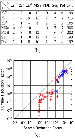
Figure 3(a) shows the coverage results. The modified Aidos configuration is indicated by "† ". The version that participated in UIPC'16 is shown on the right-hand side of the table, together with MSp and the only other online dead-end learning technique ∆C [Steinmetz and Hoffmann, 2016a]. The results for ∆-trap online learning are shown in the middle part of the table ("-" shows the results for ∆ alone, "Θ" for ∆+∆Θ). The left part shows the results for dead-end detection by ∆Θ, for offline computed ∆0 -traps Θ. The partial state candidates for the offline ∆-trap computation are chosen to all partial states of size up to k = 1, respectively k = 2. Remember that ∆0 -traps correspond exactly to the traps as originally proposed by Lipovetzky et al. [2016], and that offline ∆0 -traps are computed according to exactly that proposal. Figure 3(b) shows the effect of the different ∆ on offline computed traps for k = 2. The results for k = 1 look similar, and are left out for space reasons.
Consider first offline construction. Partial states of size 1 are not enough to compute a non-empty ∆0 -trap in any domain but DocTransfer, effectively turning the respective configuration into blind search. The computed ∆0 -traps for k = 2 help in Bottleneck, DocTransfer, and most notably in Mystery for which the initial state was already represented by the trap in every single task. As indicated by Figure 3(b), the different dead-end detectors ∆ have complementary effects on trap generation. Any one ∆ helps in some domain, yet is detrimental in others. The latter is due to the additional overhead resulting from the evaluation of such ∆ during trap construction. At the same time, ∆ does not always help to improve the computed trap. An extreme example for that is MSa, which vastly increases coverage in the resourceconstrained domains, but worsens the results on all other domains considerably. Overall, dead-end detection through an offline computed ∆-trap alone cannot compete with current state-of-the-art methods.
The potential of ∆-traps really becomes alive, however, in online learning. State-of-the-art performance is achieved in many domains even for Θ using ∆0 , i. e., without any additional dead-end detector. This vanilla configuration outperforms, in particular, the only other dead-end learning configuration ∆C in its prime discipline, the resource-constrained domains. Coverage in the latter can be increased even further through combination with the PDB heuristic, pushing the respective ∆-trap learning configuration to perfect coverage in NoMystery and Rovers. In TPP, ∆-trap learning is inferior only to Aidos' resource-variable identification component.
∆-trap learning improves overall coverage on the resourceconstrained domains for every tested ∆ except for MSa. On the other domains, the overall picture is not as consistently good. The number of domains where ∆-trap learning positively (negatively) affects coverage are 9 (7) for ∆1 ; 7 (5)
Offline Online ∆0 ∆0 ∆1 ∆2 MSa PDB Seq Pot Aidos† Domain # k=1 k=2 - Θ - Θ - Θ - Θ - Θ - Θ - Θ - Θ Aidos MSp ∆C Unsolvable Benchmarks [Hoffmann et al., 2014] 3unsat 30 15 15 15 11 15 10 15 10 10 5 15 10 20 15 20 15 15 10 30 10 5 Mystery 9 2 9 2 1 2 2 8 8 6 6 6 6 1 1 9 9 9 9 9 6 5 ∑ 39 17 24 17 12 17 12 23 18 16 11 21 16 21 16 29 24 24 19 39 16 10 UIPC'16 Benchmarks BagBarman 20 12 12 12 0 8 0 0 0 4 0 12 0 4 0 4 0 12 0 12 0 0 BagGripper 25 5 1 6 5 3 3 0 0 3 3 3 3 23 23 3 3 25 23 5 3 3 BagTransport 29 7 7 7 7 6 7 16 16 6 6 7 7 29 29 24 24 29 29 22 1 7 Bottleneck 25 10 15 10 8 20 16 21 19 10 4 19 18 25 25 25 25 25 25 25 5 9 CaveDiving 25 7 7 7 5 7 5 6 5 7 4 7 5 8 6 8 7 9 7 8 3 8 ChessBoard 23 5 5 5 3 5 3 4 3 5 2 5 3 23 23 23 23 23 23 23 2 2 Diagnosis 11 4 5 4 6 6 9 5 6 4 4 5 9 4 9 4 8 5 9 5 5 8 DocTransfer 20 6 11 5 5 7 11 7 7 10 6 12 16 6 10 7 7 15 16 13 5 5 NoMystery 20 2 2 2 11 2 11 2 8 8 9 11 13 2 11 5 6 11 13 11 11 11 Rovers 20 7 7 7 13 7 13 7 12 9 10 12 17 6 12 6 12 12 16 14 15 12 TPP 30 17 17 17 24 17 23 15 20 24 23 24 24 14 14 19 19 24 24 29 24 20 PegSol 24 24 24 24 18 24 18 21 16 24 16 24 16 24 18 22 20 24 16 24 24 14 PegSolRow5 15 5 5 5 4 5 4 4 4 5 4 5 4 15 15 15 15 15 15 15 3 4 SlidingTiles 20 10 10 10 10 10 10 10 10 10 10 10 10 10 10 10 10 10 10 10 10 10 Tetris 20 10 10 10 10 5 5 5 5 5 5 10 10 20 20 20 20 20 20 20 5 5 ∑ 327 131 138 131 129 132 138 123 131 134 106 166 155 213 225 195 199 259 246 236 116 118 Unsolvable Resource-Constrained Benchmarks [Nakhost et al., 2012] NoMystery 150 26 26 26 143 52 142 83 125 130 134 149 150 16 136 68 79 149 150 149 150 130 Rovers 150 3 3 3 142 7 139 67 120 111 111 93 150 1 125 1 125 93 150 109 129 144 TPP 25 5 8 5 19 7 21 8 9 17 12 20 21 1 1 11 11 19 21 25 16 14 ∑ 325 34 37 34 304 66 302 158 254 258 257 262 321 18 262 80 215 261 321 283 295 288 ∑ 691 182 199 182 445 215 452 304 403 408 374 449 492 252 503 304 438 544 586 558 427 416 |
(a)
Figure 3: (a) Coverage results: number of instances solved within the limits. (b) Comparison of different ∆ for ∆-trap offline construction (k=2). The table shows the number of domains on which the offline computed trap for ∆ "x" achieves higher coverage than the offline computed trap for ∆ "y", and total coverage (Cov); (c) Impact of ∆-trap online learning on the ∆0 -baseline. Per-instance based comparison of search reduction factors (x-axis) vs. runtime reduction factors (y-axis) for UIPC (+) and resource-constrained domains (x).
for ∆2 ; 3 (10) for MSa; 7 (7) for PDB; 6 (4) for Seq; 5 (4) for Pot; and 7 (5) for Aidos† . Synergistic effects, where the combination of ∆ with ∆-trap learning solves instances not solved by either of the component techniques alone, occur for PDBs in the resource-constrained domains, as well as for ∆1 , Seq, and Pot in Diagnosis and DocTransfer.
Figure 3(c) compares for every benchmark instance the search and runtime reduction factors that result from enabling trap online learning in the ∆0 -baseline (the results for other ∆ are similar). Search reduction is computed from the number of states that are visited in search. The difference between search and runtime reduction corresponds exactly to the overhead induced by trap evaluation and refinement. In the instances where runtime could not be reduced (points below 100 ), trap refinement does not generalize at sufficient scale, and thus the overhead outweighs the benefits of trap learning. Extreme examples are the various PegSol domains, for which generalization does not happen at all. In contrast, search effort is reduced by several orders of magnitude in, e. g., DocTransfer, Diagnosis, and the resource-constrained domains.
Regarding Aidos, our modified variant performs better on the UIPC domains because partial-order reduction and resource variable detection have small positive effects, yet have a large negative impact in BagGripper. Extending Aidos† by ∆-trap online learning increases overall coverage, turning it into the overall best configuration. The difference emerges from the synergies of ∆-trap learning with Aidos' components as already pointed out. Over the UIPC domains, ∆-trap learning is slightly worse overall, but its overall disadvantage is due primarily to BagBarman, where the ∆-trap generalization algorithm struggles, and often runs out of time.
8 Conclusion
Dead-end detection is an important technique in planning. One major limitation of previous dead-end detectors is transitivity, which entails that, while we can of course use as many dead-end detectors as we like, each of those is doomed to ignore the information provided by its peers. We introduce ∆-traps as a remedy, generalizing the previous trap idea to allow for synergy with a complementary dead-end detector ∆. We furthermore introduce methods allowing to learn the trap online, instead of a static offline analysis. Our experiments show that both contributions can be quite beneficial.
For future work, an aspect to look at is the generalization step in online learning, which might be optimizable for computational cost and generalization power. Beyond this, and beyond just trap learning, major questions are whether one can usefully exploit search knowledge falling short of fully identified dead-end components, and whether one can design learning methods targeted at resource limits specifically.
Acknowledgments
This work was partially supported by the German Research Foundation (DFG), under grant HO 2169/5-1, "Critically Constrained Planning via Partial Delete Relaxation", as well as by the German Federal Ministry of Education and Research (BMBF) for the Center for IT-Security, Privacy and Accountability (CISPA, grant no. 16KIS0656). Thanks to Malte Helmert for pointing out that dead-end detectors based on consistent heuristics are transitive.
| ❅ ❅ x y | ∆0 | ∆1 | ∆2 | MSa | PDB | Seq | Pot | Cov |
|---|---|---|---|---|---|---|---|---|
| ∆0 | - | 2 | 10 | 12 | 0 | 4 | 6 | 199 |
| ∆1 | 2 | - | 9 | 12 | 2 | 5 | 7 | 213 |
| ∆2 | 2 | 1 | - | 8 | 2 | 2 | 2 | 165 |
| MSa | 6 | 6 | 10 | - | 6 | 7 | 7 | 308 |
| PDB | 2 | 3 | 10 | 12 | - | 6 | 6 | 202 |
| Seq | 1 | 1 | 10 | 12 | 1 | - | 5 | 193 |
| Pot | 2 | 1 | 8 | 10 | 2 | 2 | - | 192 |
@inproceedings{ijcai2017p614,
  title     = {Search and Learn: On Dead-End Detectors, the Traps they Set, and Trap Learning},
  author    = {Steinmetz, Marcel and Hoffmann, Jörg},
  booktitle = {Proceedings of the Twenty-Sixth International Joint Conference on
               Artificial Intelligence, {IJCAI-17}},
  publisher = {International Joint Conferences on Artificial Intelligence Organization},
  editor    = {Carles Sierra, IIIA-CSIC},
  pages     = {4398--4404},
  year      = {2017},
  month     = {8},
  note      = {Main track},
  doi       = {10.24963/ijcai.2017/614},
  url       = {https://doi.org/10.24963/ijcai.2017/614},
}
TY - CPAPER TI - Search and Learn: On Dead-End Detectors, the Traps they Set, and Trap Learning AU - Steinmetz, Marcel AU - Hoffmann, Jörg T2 - Proceedings of the Twenty-Sixth International Joint Conference on Artificial Intelligence, IJCAI-17 PB - International Joint Conferences on Artificial Intelligence Organization PY - 2017 SP - 4398 EP - 4404 DO - 10.24963/ijcai.2017/614 UR - https://doi.org/10.24963/ijcai.2017/614 ER -Copied
Machine-readable versions of this paper, for tools and AI agents:





