
De-biasing Covariance-Regularized Discriminant Analysis
Proceedings of the Twenty-Seventh International Joint Conference on Artificial Intelligence. Main track. Pages 2889-2897.
https://doi.org/10.24963/ijcai.2018/401
Keywords
- Machine Learning: Data Mining
- Machine Learning Applications: Applications of Supervised Learning
Abstract
Fisher's Linear Discriminant Analysis (FLD) is a well-known technique for linear classification, feature extraction and dimension reduction. The empirical FLD relies on two key estimations from the data -- the mean vector for each class and the (inverse) covariance matrix. To improve the accuracy of FLD under the High Dimension Low Sample Size (HDLSS) settings, Covariance-Regularized FLD (CRLD) has been proposed to use shrunken covariance estimators, such as Graphical Lasso, to strike a balance between biases and variances. Though CRLD could obtain better classification accuracy, it usually incurs bias and converges to the optimal result with a slower asymptotic rate. Inspired by the recent progress in de-biased Lasso, we propose a novel FLD classifier, DBLD, which improves classification accuracy of CRLD through de-biasing. Theoretical analysis shows that DBLD possesses better asymptotic properties than CRLD. We conduct experiments on both synthetic datasets and real application datasets to confirm the correctness of our theoretical analysis and demonstrate the superiority of DBLD over classical FLD, CRLD and other downstream competitors under HDLSS settings.
- [Bickel and Levina, 2008] Peter J Bickel and Elizaveta Lev- ina. Regularized estimation of large covariance matrices. The Annals of Statistics, pages 199-227, 2008.
- [Bickel et al., 2004] Peter J Bickel, Elizaveta Levina, et al. Some theory for fisher's linear discriminant function,naive bayes', and some alternatives when there are many more variables than observations. Bernoulli, 10(6):989-1010, 2004.
- [Cai and Liu, 2011] Tony Cai and Weidong Liu. A direct estimation approach to sparse linear discriminant anal- ysis. Journal of the American Statistical Association, 106(496):1566-1577, 2011.
- [Cai et al., 2016] T Tony Cai, Zhao Ren, Harrison H Zhou, et al. Estimating structured high-dimensional covariance and precision matrices: Optimal rates and adaptive estima- tion. Electronic Journal of Statistics, 10(1):1-59, 2016.
- [DasGupta, 2008] Anirban DasGupta. Asymptotic theory of statistics and probability. Springer Science & Business Media, 2008.
- [Duda et al., 2001] Richard O. Duda, Peter E. Hart, and David G. Stork. Pattern Classification (2nd Ed). Wiley, 2001.
- [Durrant and Kabán, 2015] Robert J Durrant and Ata Kabán. Random projections as regularizers: learning a linear dis- criminant from fewer observations than dimensions. Ma- chine Learning, 99(2):257-286, 2015.
- [Friedman et al., 2008] Jerome Friedman, Trevor Hastie, and Robert Tibshirani. Sparse inverse covariance estimation with the graphical lasso. Biostatistics, 9(3):432-441, 2008.
- [Jankova et al., 2015] Jana Jankova, Sara van de Geer, et al. Confidence intervals for high-dimensional inverse covari- ance estimation. Electronic Journal of Statistics, 9(1):1205- 1229, 2015.
- [Javanmard and Montanari, 2014] Adel Javanmard and An- drea Montanari. Confidence intervals and hypothesis test- ing for high-dimensional regression. Journal of Machine Learning Research, 15(1):2869-2909, 2014.
- [Kaski and Peltonen, 2003] Samuel Kaski and Jaakko Pelto- nen. Informative discriminant analysis. In ICML, pages 329-336, 2003.
- [Krzanowski et al., 1995] WJ Krzanowski, Philip Jonathan, WV McCarthy, and MR Thomas. Discriminant analysis with singular covariance matrices: methods and applica- tions to spectroscopic data. Applied Statistics, pages 101- 115, 1995.
- [Kulis and others, 2013] Brian Kulis et al. Metric learning: A survey. Foundations and Trends in Machine Learning, 5(4):287-364, 2013.
- [Lin, 2017] Chih-Jen Lin. Libsvm data: Classification (binary class). https://www.csie.ntu.edu. tw/ ˜cjlin/libsvmtools/datasets/binary. html, 2017. Link
- [Marčenko and Pastur, 1967] Vladimir A Marčenko and Leonid A Pastur. Distribution of eigenvalues for some sets of random matrices. Mathematics of the USSR-Sbornik, 1(4):457, 1967.
- [Peck and Van Ness, 1982] Roger Peck and John Van Ness. The use of shrinkage estimators in linear discriminant anal- ysis. IEEE Transactions on Pattern Analysis and Machine Intelligence, (5):530-537, 1982.
- [Rothman et al., 2010] Adam J Rothman, Elizaveta Levina, and Ji Zhu. Sparse multivariate regression with covari- ance estimation. Journal of Computational and Graphical Statistics, 19(4):947-962, 2010.
- [Shao et al., 2011] Jun Shao, Yazhen Wang, Xinwei Deng, Sijian Wang, et al. Sparse linear discriminant analysis by thresholding for high dimensional data. The Annals of Statistics, 39(2):1241-1265, 2011.
- [Tibshirani et al., 2002] Robert Tibshirani, Trevor Hastie, Balasubramanian Narasimhan, and Gilbert Chu. Diagnosis of multiple cancer types by shrunken centroids of gene ex- pression. Proceedings of the National Academy of Sciences, 99(10):6567-6572, 2002.
- [Witten and Tibshirani, 2009] Daniela M Witten and Robert Tibshirani. Covariance-regularized regression and classi- fication for high dimensional problems. Journal of the Royal Statistical Society: Series B (Statistical Methodol- ogy), 71(3):615-636, 2009.
- [Witten et al., 2011] Daniela M Witten, Jerome H Friedman, and Noah Simon. New insights and faster computations for the graphical lasso. Journal of Computational and Graphical Statistics, 20(4):892-900, 2011.
- [Ye et al., 2004] Jieping Ye, Ravi Janardan, and Qi Li. Two- dimensional linear discriminant analysis. In NIPS, pages 1569-1576, Cambridge, MA, USA, 2004.
- [Zhang and others, 2003] Zhihua Zhang et al. Learning met- rics via discriminant kernels and multidimensional scaling: Toward expected euclidean representation. In ICML, vol- ume 2, pages 872-879, 2003.
- [Zhang and Zhang, 2014] Cun-Hui Zhang and Stephanie S Zhang. Confidence intervals for low dimensional param- eters in high dimensional linear models. Journal of the Royal Statistical Society: Series B (Statistical Methodol- ogy), 76(1):217-242, 2014.
- [Zhang et al., 2015] Jinghe Zhang, Haoyi Xiong, Yu Huang, Hao Wu, Kevin Leach, and Laura E. Barnes. MSEQ: Early detection of anxiety and depression via temporal orders of diagnoses in electronic health data. In BigData. IEEE, 2015.
- [Zollanvari and Dougherty, 2013] Amin Zollanvari and Ed- ward R Dougherty. Random matrix theory in pattern clas- sification: An application to error estimation. In 2013 Asilomar Conference on Signals, Systems and Computers, 2013.
References were extracted automatically from the PDF and may contain errors.
Full text extracted automatically from the PDF; figures, tables and equations may differ. The PDF is the version of record.
1 Introduction
Fisher's Linear Discriminant Analysis (FLD) [Duda et al., 2001] is a well-known technique for feature extraction and dimension reduction [Kulis and others, 2013]. It has been widely used in many applications, such as face recognition [Peck and Van Ness, 1982], image retrieval, etc. An intrinsic limitation of classical FLD is that its objective function relies on the well-estimated and non-singular covariance matrices. For many applications, such as the micro-array data analysis, all scatter matrices can be singular or ill-posed since the data is often with high dimension but low sample size (HDLSS) [Cai et al., 2016].
The classical FLD classifier relies on two key parameters - the mean vector of each type and the precision matrix. Under the HDLSS settings, the sample precision matrix (a.k.a., the inverse of sample covariance matrix) used in FLD is usually ill-estimated and quite different from the inverse of population/true covariance matrix [Cai et al., 2016]. For example, the largest eigenvalue of the sample covariance matrix is not a consistent estimate of the largest eigenvalue of the population covariance matrix, and the eigenvectors of the sample covariance matrix can be nearly orthogonal to the truth when the number of dimensions is greater than the number of samples [Marˇcenko and Pastur, 1967]. Such inconsistency between the true and the estimated precision matrices degrades the accuracy of FLD classifiers under the HDLSS settings [Zollanvari and Dougherty, 2013].
A plethora of excellent work has been conducted to address such HDLSS data classification problem for FLD. For example, Krzanowski et al. [Krzanowski et al., 1995] suggested to use pseudo-inverse to approximate the inverse covariance matrix, when the sample covariance matrix is singular. However, the precision of pseudo-inverse FLD is usually low and not well guaranteed. Other techniques include the two-stage algorithm PCA+FLD [Ye et al., 2004], FLD based on Kernels [Zhang and others, 2003] and/or other nonparametric statistics [Kaski and Peltonen, 2003]. To overcome the singularity of the sample covariance matrices, instead of estimating inverse covariance matrix and mean vectors separately, [Cai and Liu, 2011] proposed to estimate the projection vector for discrimination directly. More popularly, regularized FLD approaches [Krzanowski et al., 1995; Witten and Tibshirani, 2009] are proposed to solve the problem. These methods can improve the performance of FLD either empirically or theoretically [Durrant and Kab´an, 2015; Bickel et al., 2004], while few of them can directly address the ill-estimated inverse covariance matrix estimation issue.
One representative regularization approach is CovarianceRegularized FLD [Witten and Tibshirani, 2009] that replaces the precision matrix used in FLD with a shrunken estimator, such as Graphical Lasso [Friedman et al., 2008], so as to achieve a "superior prediction". Intuitively, through replacing precision matrix used in FLD with a sparse regularized estimation, the ill-posed problem caused by the HDLSS settings can be well addressed. The sparse estimators usually converge to the inverse of true/population covariance matrix faster than the sample estimators [Cai et al., 2016]. With the asymptotic properties, the sparse FLD should be close to the optimal FLD. However, the way that the sparsity and the convergence rate of the precision matrix estimator would affect the classification accuracy is not well studied in literature.
Further, with induced sparsity, the inverse covariance estimator becomes biased [Zhang and Zhang, 2014]. The performance of sparse FLD is frequently bottlenecked due to the bias of the sparse estimators. Recently, researchers tried to de-bias the Lasso estimator [Zhang and Zhang, 2014], through adjusting the ℓ1-penalty for the regularized estimation, so as to achieve a better regression performance. Inspired by this line of research, we propose to improve sparse FLD through de-biasing (i.e., de-sparsifing) in this paper.
Our Contributions. With respect to the aforementioned issues, in this paper, we made the following contributions.
- Inspired by De-biased Lasso [Javanmard and Montanari, 2014], we study the problem of de-biasing the Covariance-Regularized FLD (CRLD), which has been widely-used for empirical sparse FLD estimation, for performance improvement. To the best of our knowledge, this is the first work aiming at de-biasing CRLD.
- We propose a novel algorithm DBLD - De-Biased Fisher's Linear Discriminant Analysis on top of CRLD. DBLD leverages yet-another De-Biased Estimator for linear classification problem, to re-balance the variances and biases of the estimation, through de-sparsifying the projection vector obtained by CRLD.
- Our theoretical analysis shows, under certain mild assumptions, DBLD converges faster than CRLD with sharp asymptotic rate. We also conduct extensive experiments to demonstrate the advantage of the proposed algorithms over other competitors. The results validate the correctness of our theoretical analysis.
Notations. Following key notations are used in the rest of this paper: Given a p-dimensional vector v ∈ Rp , we denote the ℓP vector-norm as |v|P = (∑mi=1 |vi|P )1/P (P is a non-negative integer) and the ℓ∞ vector-norm as |v|∞ = max1≤i≤m{|vi|}. Given a matrix A ∈ Rm1×m2 , we denote the ℓP matrix-norm as ||A||P = maxv∈Rp{|Av|P/|v|P}. Note that the symbol p refers to the number of dimensions of the data while m refers to the number of samples. The operator Op(·) refers to the big-O-notation in high probability.
2 Preliminaries
In this section, we first briefly introduce the binary classifier using FLD, then present the practice of CRLD based on Graphical Lasso.
2.1 FLD for Binary Classification
To use the Fisher's Linear Discriminant Analysis (FLD), given the i.i.d. labeled data pairs (x1, ℓ1) . . . (xm, ℓm), we first estimate the sample covariance matrix ¯Σ using the pooled sample covariance matrix estimator with respect to the two classes [Duda et al., 2001], then estimate the sample precision matrix as ¯Θ = ¯Σ-1 . Further, ¯µ+ and ¯µ- are estimated as the mean vectors of the positive samples and the negative samples in the m training samples, respectively.
Given all estimated parameters ¯Σ (and ¯Θ = ¯Σ-1 ), ¯µ+ and ¯µ-, the FLD model classifies a new data vector x as the result of:
where π+ and π- refer to the (foreknown) frequencies of positive samples and negative samples in the whole population, respectively.
2.2 Covariance-Regularized FLD via Graphical Lasso
This algorithm, referred to as the Covariance-Regularized FLD (CRLD) via Graphical Lasso, was derived from the Scout family of FLD introduced by Witten et al. in [Witten and Tibshirani, 2009]. Compared to the classical FLD, this baseline algorithm leverages Graphical Lasso estimator to replace the precision matrix estimated using sample covariance matrix. The proposed algorithm is implemented using the discriminant function defined in Eq. 1, as:
where ̂Θ refers to the Graphical Lasso estimator based on the sample covariance matrix ¯Σ:
Note that, as a linear classifier, the CRLD decision rule introduced in Eq. 2 can be re-formulated in a linear model, such as:
where sign(·) function returns +1 if the input is non-negative, and -1 when the input is negative. The vector ̂ βG = ̂Θ(¯µ+ - ¯µ-) and the scalar cg = - 12 · (¯µ+ + ¯µ-)⊤̂ βG + log(π+/π-). Obviously, ̂ βG is the vector of projection coefficients for linear classification.
In this paper, we present the analytical results (i.e., statistical rate of convergence that ̂ βG approximates to the optimal projection vector with varying number of samples n and dimensions p) of CRLD in Theorem 1.
3 The Proposed Algorithm
In this section, we introduce our proposed algorithmDBLDDe-Biased Fisher's Linear Discriminant Analysis (via Graphical Lasso), then present the theoretical analysis on the theoretical properties of the proposed algorithms.
3.1 DBLD: The De-Biased Estimation for Covariance-Regularized FLD
Given the i.i.d. labeled data pairs (x1, ℓ1) . . . (xm, ℓm) drawn from the two classes with certain priors, as shown in Algorithm 1. The algorithm first (i) estimates the sample estimation of covariance matrices and the mean vectors, then (ii) leverages CRLD to estimate the shrunken projection vector ̂ βG. Further, DBLD (iii) proposes a de-biased estimator (denoted as DeBias function) to de-bias ̂ βG and obtain the projection vector ̂ βD . Finally, we introduce a decision rule that enables classification using the estimated ̂ βD .
Algorithm 1 DBLD Estimation Algorithm
- 1: procedure DBLD((x1, ℓ1) . . . (xm, ℓm))
- 2: /*(i) Sample Estimators for Mean and Covariance */
- 3: X+ ←PositiveSampleSet((x1, ℓ1)..(xm, ℓm));
- 4: X- ←NegativeSampleSet((x1, ℓ1)..(xm, ℓm));
5:
6:
¯µ+ ← 1
|X+| · ∑x∈X+ x, ¯µ- ← 1
¯Σ+ ← 1
|X-| · ∑x∈X- x;
|X+| · ∑x∈X+ (x- ¯µ+)(x- ¯µ+)⊤;
8:
¯µ ← |X+|·¯µ++|X-|·¯µ-
|X+|+|X-|
, ¯Σ← |X+|·¯Σ++|X-|·¯Σ-
|X+|+|X-|
- 9: /*(ii) CRLD Estimator (to obtain ̂ βG) */
10: ̂Θ←GraphicalLasso(¯Σ, λ);
11: ̂
βG ← ̂Θ(¯µ+ - ¯µ-);
- 12: /*(iii) DBLDEstimator (to obtain ̂ βD ) */
13: X← [x1, x2, ...xm]; /*p×mmatrix */
14: L← [ℓ1, ℓ2, . . . ℓm]⊤; /*m×1 matrix */
- 15: U← [¯µ, ¯µ, . . . ¯µ];
- 16: /*U is an m× p matrix, every column is ¯µ*/
- 17: c ← -¯µ⊤ ̂ βG;
- 18: C← [c, c, . . . , c]⊤;
- 19: /*C is a m × 1 matrix, every row is c*/
- 21: return ̂ βD ;
In the following section, we present the design of the DeBiased Estimator (denoted as DeBiasing function in Algorithm 1) to obtain ̂ βD , then introduce the decision rule for optimal classification. Later we analyze the theoretical properties of ̂ βD .
The De-Biased Estimator
Inspired by the De-biased Lasso [Javanmard and Montanari, 2014], we propose to improve the performance of CRLD through de-biasing βG. Given m labeled training data (x1, ℓ1), (x2, ℓ2), . . . (xm, ℓm) with balanced labels, the Graphical Lasso estimator ̂Θ on the data and the CRLD model (i.e., ˆ βG), we propose a novel de-biased estimator of ˆ βD that takes the form as
where we denote X as an p × m matrix where 1 ≤ i ≤ m and the ith column is xi; L as an m× 1 matrix (i.e., vector) whose ith row is ℓi ∈ {±1}; U is a p × m matrix where each column is ¯µ (as line 7 in Algorithm 1); and C is an m× 1 matrix where each row is c (as line 16 in Algorithm 1).
;
The DBLD Classifier.
Given the de-biased estimator ̂ βD , the DBLD classifies the input vector x using the following rule:
In the following section, we present the analytical results of DBLD, including the computational complexity of debiasing and statistical rate of convergence.
3.2 Complexity Analysis of DBLD
In this section, we analyze the computational complexity for the three steps of Algorithm 1. The step (i) estimates the sample covariance matrices and mean vectors, which consumes at most O(p2 · m) operations. The step (ii) performs Graphical Lasso and matrix multiplication, where the complexity based on standard implementation [Friedman et al., 2008] is upperbounded by O(p3 ). The step (iii) de-biasing is implemented as an exact formula with O(p2 ) complexity.
Remark 1. All three steps of Algorithm 1 are scalable on both the number of dimensions (p) and the number of training samples (m). The overall complexity of the three steps is O(p3 + p2 · m). Under the HDLSS setting p > m, the computational complexity of DBLD is upper-bounded by O(p3 ). On the other hand, with large sample setting where m ≥ p, the worst case computational complexity of DBLD is bounded by O(p2 · m). Obviously, the proposed de-biasing estimator (i.e., step (iii)) with complexity O(p2 ) would not bound the performance, when compared to the first two steps.
3.3 Convergence Analysis of DBLD
In order to analyze the performance of DBLD, we first define the linear projection vector of the optimal FLD as β∗ . Given m samples (x1, ℓ1), . . . (xm, ℓm) drawn i.i.d. from N(µ∗+,Σ∗ ) and N(µ∗-,Σ∗ ) with the equal priors for training, the optimal projection vector should be β∗ = Θ∗ (µ∗+ - µ∗-) and Θ∗ = Σ∗-1 . We intend to understand how close ̂ βG and ̂ βD approximate to the optimal estimation β∗ .
Assumption 1. We follow the assumptions made in [Rothman et al., 2010] that a positive constant K having
exists. The operators λmin(·) and λmax(·) denote the smallest and largest eigenvalues respectively. In this way, there exists ‖Σ∗ ‖2 ≤ K and ‖Θ∗ ‖2 ≤ K.
Assumption 2. We further follow the assumption that, the data vectors for training are all realized from a random vector X and there exists an constant B having |X|2 ≤ B. Thus there has |¯µ+|2 ≤ B and |¯µ-|2 ≤ B.
Theorem 1. With appropriate setting of tuning parameter λ ≍ √logp/m (in Eq 3), the ℓ2-vector-norm convergence rate of CRLD ̂ βG approximating to the optimal estimation β∗ is:
where d = max1≤i≤p|{j : Σ∗-1 i,j ̸= 0}| refers to the maximal degree of the graph (i.e., population inverse covariance matrix).
Proof. Here, we first prove the upper bound of |̂ βG - β∗ |∞. As was defined ̂ βG = ̂Θ(¯µ+ - ¯µ-), then we have:
Considering the inequities |x+y|2 ≤ |x|2 +|y|2 and |Ax|2 ≤ ||A||2 · |x|2, we have
According to [Rothman et al., 2010], when λ ≍ √logp/m, we consider the spectral-norm convergence rate ‖̂Θ-Θ∗ ‖2 ≤ ‖̂Θ-Θ∗ ‖F = Op(√(p+d) · log p/m), the asymptotic rate of sample mean vector [DasGupta, 2008] is |¯µ+ - µ∗+|2 = Op(√p/m) and |¯µ--µ∗-|2 = Op(√p/m), with the increasing number of dimensions p and number of samples m.
Further, there has ‖Θ∗ ‖2 ≤ K (Assumption 1) and ℓ2norms of all mean vectors are bounded by B. In this way, there must exist positive constants C1 and C2 having:
Thus, according to the definition of asymptotic rate, we conclude the convergence rate as:
Theorem 2. With appropriate setting of tuning parameter λ (in Eq 3), the ℓ2-vector-norm convergence rate of DBLD ̂ βG approximating to the optimal estimation β∗ is:
Proof. Here, we prove the upper bound of |̂ βD - β∗ |∞. Consider the definition of the de-biased FLD estimator ̂ βD introduced in Eq. 5, we have
With the assumption of equal priors (π+ = π- = 0.5), L is a m× 1 label matrix that half of its elements are +1 while the rest are all -1. X refers to a p×m matrix, where each column is a sample of data e.g., x1, x2, . . . , xm. As was defined ̂ βG = ̂Θ(¯µ+ - ¯µ-) = 2m · ̂ΘXL. As U is a matrix in which each column is a constant vector (¯µ+ + ¯µ-)/2 and L is a vector with half elements as 1 and half elements as -1, thus 2m ·
̂ΘUL = 2m · ̂Θ(UL) = 0. As each column of X refers to a sample drawn from the original data distribution, thus 1m (X-U)(X-U)⊤ = ¯Σs is the sample covariance matrix estimator. With all above in mind, we have
where I refers to a p × p identity matrix. Note that (I - ̂Θ¯Σ) ̂ βG can be considered as the de-sparsification term that de-biases ̂ βG. Thus, considering the asymptotic rate of sample mean vector [DasGupta, 2008] is |¯µ+ - µ∗+|2 = Op(√p/m) and |¯µ- - µ∗-|2 = Op(√p/m), we have
According to [Jankova et al., 2015], with appropriate setting of λ, the spectral-norm convergence rate of the de-sparisified estimator ̂ΘD = (2 · ̂Θ- ̂Θ¯Σs ̂Θ) under mild conditions should be ‖̂ΘD -Θ∗ ‖∞ = Op(√log p/m), then there exists ‖̂ΘD - Θ∗ ‖2 = Op(√p log p/m), with the varying number of dimensions p and number of samples m. In this way, with high probability, we conclude the convergence rate:
Remark 2. Compared to CRLD's projection vector ̂ βG, our method DBLD recovers the linear projection vector ̂ βD with a faster asymptotic rate, i.e., √p log p/m v.s. √(p + d) log p/m in a mild condition. Thus, it would benefit to some applications, such as dimensionality reduction and feature selection. Our later experimental results show that DBLD outperforms CRLD with higher classification accuracy, due to the faster statistical rate of convergence.
Remark 3. The proposed algorithm provides a sub-optimal solution, when compared to [Cai and Liu, 2011]. Our work intend to propose an estimator of β∗ through approximating Σ∗ , µ∗+ and µ∗- separately, while [Cai and Liu, 2011] approximates ̂ β∗ straightforwardly via so-called "direct estimation".
4 Experiments
In this section, we first validate different properties of DBLD on the synthesized data. Then, we experimentally evaluate the performance of DBLD using several real-world datasets. Experiments show the superiority of DBLD.
4.1 Synthesized Data Evaluation
To validate our algorithms, we evaluate our algorithms on a synthesized dataset (imported from [Cai and Liu, 2011]), which is obtained through a pseudo-random simulation. The synthetic data are generated by two predefined Gaussian distributions N(µ∗+, Σ∗ ) and N(µ∗-, Σ∗ ) with equal priors. The settings of µ∗+, µ∗- and Σ∗ are as follows: Σ∗ is a p×p symmetric and positive-definite matrix, where each element Σ∗i,j = 0.8|i-j| , 1 ≤ i ≤ p and 1 ≤ j ≤ p. µ∗+ and µ∗- are both pdimensional vectors, where µ∗+ = 〈1, 1, . . . , 1, 0, 0, . . . , 0〉T (the first 10 elements are all 1's, while the rest p-10 elements are 0's) and µ∗- = 0. In our experiment, we set p = 200. To simulate the HDLSS settings, we train CRLD and DBLD, with 20 to 200 samples randomly drawn from the distributions with equal priors, and test the two algorithms using 500 randomly generated samples. For each settings, we repeat the experiments for 100 times and report the averaged results, in a cross-validation manner.
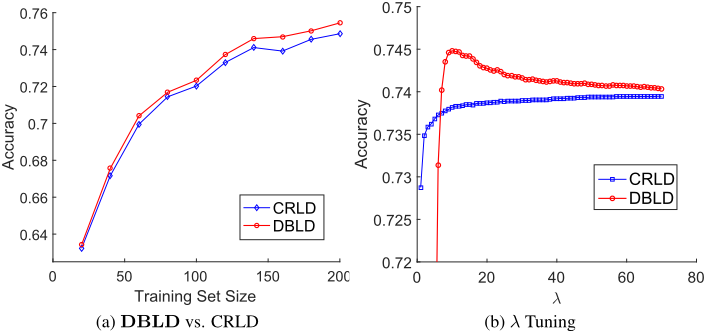
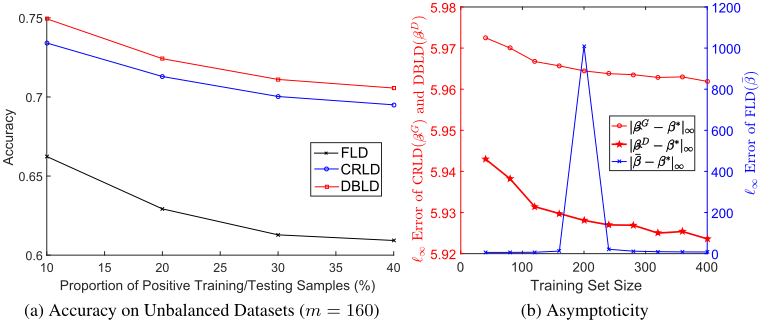
In this experiment, we compare DBLD, CRLD and FLD (with pseudo inverse). The results of FLD is not included here, as it performs extremely worse than both CRLD and DBLD under the HDLSS settings. Figure. 1(a) presents the comparison between DBLD and CRLD, in terms of accuracy, where each algorithm is fine tuned with the best parameter λ. A detailed example of parameter tuning is reported in Figure. 1(b), where we run both algorithms, with training set size as 160, when varying λ from 1 to 70. From Figure. 1(a), it is obvious that DBLD outperforms CRLD marginally. The λ tuning comparison addressed in Figure. 1(b) shows that, given a small λ, both CRLD and DBLD cannot perform well, as the sparse approximation of ̂ βG and ̂ βD cannot be well recovered in such case [Witten and Tibshirani, 2009]. When λ ≥ 6, DBLD starts outperforming CRLD, while the advantage of DBLD to CRLD decreases when increasing λ. However, even with an extremely large λ, DBLD still outperforms CRLD. In Figure 2(a), we present the evaluation results based on unbalanced datasets, where the accuracy of algorithms using m = 160 training samples drawn with varying priors is illustrated. The proportion of positive training samples is varying from 10% to 40%. It is obvious that all algorithms achieve their best performance when the proportion of positive training sample is 10% (the most unbalanced case).
To further verify our algorithms, we propose the optimal FLD classifier β∗ = Θ∗ (µ∗+ - µ∗-), which is all based on the population parameters. We compare the ̂ βD , ̂ βG and ¯ β estimated by DBLD, CRLD and FLD (with pseudo-inverse) to β∗ . Figure. 2(b) presents the comparison among |̂ βD - β∗ |∞, |̂ βG-β∗ |∞ and | ¯ β-β∗ |∞. It is obvious that ̂ βD is more close to β∗ than ̂ βG and ¯ β. This observation further verifies the Theorem 1 and 2. We also compare the accuracy of β∗ to CRLD, DBLD and FLD. β∗ outperforms these algorithms and the accuracy of β∗ is around 84.4% It is reasonable to conclude that DBLD outperforms CRLD, because ̂ βD is more close to β∗ .
4.2 Benchmark Evaluation Results
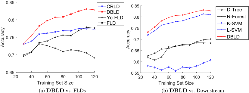
In Figure. 3(a), we compare DBLD and other FLD algorithms, including FLD with pseudo-inverse, Sparse FLD via Graphical Lasso (CRLD) and Ye-FLD derived from [Ye et al., 2004], on the Web datasets [Lin, 2017]. To simulate the HDLSS settings (p ≫ m), we vary the training sample sizes from 30 to 120 while using 400 samples for testing. The numbers of dimensions p is 300. For each algorithm, reported result is averaged over 100 randomly selected subsets of the training/testing data with equal priors. CRLD and DBLD are fine-tuned with the best λ. The experimental settings show that DBLD consistently outperforms other competitors in different settings. The non-monotonic trend of FLD with the increasing training set size is partially due to the poor performance of pseudo inverse used in FLD.
In addition to FLD classifiers, we also compared DBLD with other downstream algorithms including Decision Tree, Random Forest, Linear Support Vector Machine (SVM) and Kernel SVM with Gaussian Kernel. The comparison results are listed in Figure. 3(b). All algorithms are fine-tuned with the best parameters under our experiment settings.
4.3 Early Detection of Diseases on EHRDatasets
To demonstrate the effectiveness of DBLD in handling the real problems, we evaluate DBLD on the real-world Electronic Health Records (EHR) data for early detection of dis-
`1 Error of FLD(-7)
| Training Set Size | |||||||
|---|---|---|---|---|---|---|---|
| Algorithm | 100 | 200 | 300 | 400 | 500 | 600 | 700 |
| DBLD | 0.659±0.022 | 0.677±0.028 | 0.691±0.024 | 0.692±0.023 | 0.690±0.021 | 0.696±0.024 | 0.701±0.023 |
| FLD | 0.543±0.034 | 0.586±0.033 | 0.616±0.022 | 0.642±0.029 | 0.642±0.022 | 0.657±0.025 | 0.658±0.026 |
| Ye-FLD | 0.627±0.050 | 0.620±0.077 | 0.652±0.063 | 0.620±0.067 | 0.655±0.062 | 0.637±0.064 | 0.670±0.045 |
| Decision Tree | 0.621±0.046 | 0.649±0.031 | 0.652±0.041 | 0.655±0.030 | 0.671±0.028 | 0.665±0.031 | 0.668±0.040 |
| Linear SVM | 0.615±0.026 | 0.628±0.030 | 0.647±0.023 | 0.666±0.029 | 0.666±0.021 | 0.670±0.030 | 0.675±0.029 |
| Kernel SVM | 0.635±0.032 | 0.669±0.027 | 0.674±0.039 | 0.678±0.021 | 0.668±0.038 | 0.688±0.024 | 0.682±0.029 |
| AdaBoost | 0.631±0.035 | 0.630±0.039 | 0.620±0.028 | 0.622±0.027 | 0.621±0.022 | 0.617±0.025 | 0.626±0.070 |
| CRLD | 0.658±0.023 | 0.676±0.024 | 0.682±0.028 | 0.686±0.022 | 0.683±0.021 | 0.692±0.025 | 0.695±0.018 |
| Random Forest | 0.590±0.035 | 0.602±0.035 | 0.653±0.031 | 0.602±0.040 | 0.674±0.024 | 0.666±0.026 | 0.658±0.032 |
eases [Zhang et al., 2015]. In this application, each patient's EHR data is represented by a p = 295 dimensional vector, referring to the outpatient record on the physical disorders diagnosed. Patients are labeled with either "positive" or "negative", indicating whether he/she was diagnosed with depression & anxiety disorders. Through supervised learning on the datasets, the trained binary classifier is expected to predict whether a (new) patient is at-risk or would develop to the depression & anxiety disorders from their historical outpatient records (physical disorder records) [Zhang et al., 2015].
| Training Set | |||||||
|---|---|---|---|---|---|---|---|
| Algorithm | 100 | 200 | 300 | 400 | 500 | 600 | 700 |
| DBLD | 0.690±0.028 | 0.708±0.027 | 0.722±0.024 | 0.729±0.018 | 0.727±0.0118 | 0.736±0.018 | 0.734±0.022 |
| FLD | 0.539±0.048 | 0.580±0.044 | 0.611±0.030 | 0.646±0.027 | 0.644±0.025 | 0.662±0.028 | 0.663±0.032 |
| Ye-FLD | 0.644±0.100 | 0.657±0.124 | 0.688±0.071 | 0.678±0.057 | 0.698±0.035 | 0.698±0.035 | 0.712±0.027 |
| Decision Tree | 0.626±0.120 | 0.671±0.074 | 0.675±0.088 | 0.703±0.032 | 0.695±0.034 | 0.676±0.078 | 0.690±0.097 |
| Linear SVM | 0.616±0.031 | 0.627±0.041 | 0.651±0.026 | 0.675±0.031 | 0.675±0.026 | 0.680±0.035 | 0.690±0.031 |
| Kernel SVM | 0.701±0.063 | 0.723±0.022 | 0.702±0.115 | 0.726±0.016 | 0.681±0.115 | 0.734±0.019 | 0.715±0.071 |
| AdaBoost | 0.560±0.081 | 0.533±0.107 | 0.498±0.065 | 0.503±0.078 | 0.500±0.080 | 0.482±0.066 | 0.503±0.070 |
| CRLD | 0.696±0.021 | 0.716±0.021 | 0.719±0.024 | 0.725±0.018 | 0.721±0.015 | 0.733±0.021 | 0.734±0.016 |
| Random Forest | 0.419±0.126 | 0.509±0.102 | 0.613±0.067 | 0.509±0.110 | 0.661±0.036 | 0.640±0.058 | 0.603±0.063 |
| Datasets | # Features | # Samples |
| Leukemia | 7,128 | 72 (47 / 25) |
| Colon | 2,000 | 62 (40 / 22) |
We evaluate DBLD and other competitors, including Linear Support Vector Machine, Nonlinear SVM with Gaussian Kernel, Decision Tree, AdaBoost, Random Forest and other FLD baselines, with varying training dataset size m from 100 to 700. Table 1 presents the comparison results. To simplify the comparison, we only present the results of the algorithm with fine-tuned parameter, which is selected through 10-fold cross-validation. It is obvious that DBLD and CRLD outperform other baseline algorithms significantly, while DBLD performs better than CRLD. The advantage of DBLD over other algorithms, such as SVM, is extremely obvious when the size of training dataset m is small. With the increasing sample size, though the margins of DBLD over the rest of algorithms decrease, DBLD still outperforms other algorithms. We also measured the F1-score of all algorithms, DBLD still outperforms other competitors in the most cases. Please refer to Table 2 for details.
4.4 Leukemia and Colon Cancer Datasets
We evaluate DBLD, CRLD and other baseline algorithms, including Decision Tree, Random Forest and SVM, using leukemia and colon cancer datasets (derived from [Lin, 2017; Tibshirani et al., 2002]) under HDLSS settings (i.e., p = 7, 128 and 2, 000 vs. m = 20).
Table ?? presents the description of two datasets [Lin, 2017; Tibshirani et al., 2002] that we used to evaluate the proposed and baseline algorithms. "Leukemia" refers to the leukemia cancer dataset [Tibshirani et al., 2002] that includes 7,128 features and totally 72 samples (for training and testing). In this datasets, 47 samples are labeled as "ALL" class while 25 samples are identified as "AML". On the other hand, "Colon" refers to the colon cancer datasets [Lin, 2017] that are with 2,000 features and totally 62 samples, where 40 samples are negative and 22 samples are identified as positive. Both datasets are with a ultra-large number of dimensions but with extremely low sample sizes (i.e., p ≫ m).
To accurately estimate the performance of algorithms using these datasets under HDLSS settings, we use cross-validation to limit the potential over-fitting. In each round of crossvalidation, we first randomly drawn 20 samples with equal prior from the datasets as the training set, and randomly drawn 20 samples with equal prior from the disjoint set of training set as the testing set. For each round of cross validation, there are no common samples shared by the two sets. We use the training set to train each classifier (i.e., p = 7, 128 or 2, 000 and m = 20 ), so as to simulate the extremely HDLSS settings, then test the trained classifiers using the testing set. For each experiment, we repeat the cross-validation for 100 rounds. All algorithms (including baselines and DBLD) are tuned to have the best accuracy. The experiment results are shown in Table ??. All results show that DBLD significantly improves CRLD, and it outperforms all baseline algorithms with the highest accuracy and F1-score. Please note that though we trained classifiers using less training data, baselines in our experiments perform comparably with the test errors reported in [Tibshirani et al., 2002].
4.5 Summary of Experiment Results
We evaluate DBLD with a limited number of samples for training i.e., p > m or m ̸≫ p, to understand its performance under HDLSS setting. For large sample scenario, i.e., when m ≫ p, the sample-based estimators may provide a robust estimation of LDA. In this case, singularity issues might not exist, then regularization and further the de-biasing procedures are not mandatory.
| Colon | Leukemia | |||
|---|---|---|---|---|
| Algorithm | Accuracy | F1 Score | Accuracy | F1 Score |
| DBLD | 0.803 | 0.802 | 0.964 | 0.964 |
| CRLD | 0.633 | 0.630 | 0.690 | 0.690 |
| Decision Tree | 0.669 | 0.658 | 0.804 | 0.800 |
| Random Forest | 0.801 | 0.798 | 0.957 | 0.956 |
| SVM | 0.797 | 0.812 | 0.906 | 0.914 |
5 RelatedWork and Discussion
In this section, we review several most relevant studies of our research. To address the HDLSS issues for FLD, a line of research [Shao et al., 2011; Cai and Liu, 2011] proposed to directly estimate a sparse projection vector without estimating the inverse covariance matrix (sample covariance matrix is not invertible) and mean vectors separately. On the other hand, [Peck and Van Ness, 1982; Bickel and Levina, 2008; Witten and Tibshirani, 2009] proposed to first estimate the inverse covariance matrix through shrunken covariance estimators, then estimate the projection vector with sample mean vectors. Through regularizing the (inverse) covariance matrix estimation, these algorithms are expected to estimate a sparse projection vector with (sub-)optimal discrimination power [Zollanvari and Dougherty, 2013]. Moreover, the performance of FLD has been previously studied in [Durrant and Kab´an, 2015; Bickel et al., 2004].
In our paper, we focus on improving covariance-regularized FLD [Witten and Tibshirani, 2009], through de-biasing the projection vector estimated with Graphical Lasso [Witten et al., 2011]. Our work is distinct due to the following reasons: (1) Our work is the first to study the problem of de-biasing the sparse FLD [Zhang and Zhang, 2014]; (2) Compared to the existing solution to the de-biased linear regression models [Javanmard and Montanari, 2014], we proposed a novel de-biased estimator (using a different formulate in Eq 5) for the covariance-regularized sparse Linear Discriminant Analysis [Witten and Tibshirani, 2009; Witten et al., 2011]; (3) We analyzed the de-biased estimator and obtained its asymptotic properties; (4) We validate our algorithms through comparing a wide range of baselines on both synthesized and real-world datasets, where the evaluation result endorses our theory (e.g., asymptotic properties proved in Theorem 1 and 2 vs. the curve shown in Fig 2(b)).
Discussion and Future Work. In this research, we compare DBLD with CRLD, and common FLD (sample FLD, pseudo-inverse FLD, Ye-FLD). We do not make further comparison with other sparse FLD [Cai and Liu, 2011], as we focus on the covariance-regularization. In future work, we plan to study the de-biased estimators for these sparse FLD.
6 Conclusion
In this paper, we studied the problem of improving the performance of covariance-regularized FLD (CRLD) through re-balancing the biases and variances of the projection vector estimation. Inspired by the de-biased estimator of Lasso [Javanmard and Montanari, 2014], we proposed DBLD - a novel De-Biased estimator for CRLD that lowers the estimation error with faster asymptotic rate, through de-biasing the projection vector obtained by CRLD. Our analysis shows that DBLD is with better asymptotic properties, compared to CRLD, and can obtain higher classification accuracy, under HDLSS settings. The experimental results on synthesized and real-world datasets show that DBLD outperformed all baseline algorithms. Further, the empirical studies on estimator comparison validate our theoretical analysis.
@inproceedings{ijcai2018p401,
  title     = {De-biasing Covariance-Regularized Discriminant Analysis},
  author    = {Xiong, Haoyi and Cheng, Wei and Fu, Yanjie and Hu, Wenqing and Bian, Jiang and Guo, Zhishan},
  booktitle = {Proceedings of the Twenty-Seventh International Joint Conference on
               Artificial Intelligence, {IJCAI-18}},
  publisher = {International Joint Conferences on Artificial Intelligence Organization},
  editor    = {Jérôme Lang},
  pages     = {2889--2897},
  year      = {2018},
  month     = {7},
  note      = {Main track},
  doi       = {10.24963/ijcai.2018/401},
  url       = {https://doi.org/10.24963/ijcai.2018/401},
}
TY - CPAPER TI - De-biasing Covariance-Regularized Discriminant Analysis AU - Xiong, Haoyi AU - Cheng, Wei AU - Fu, Yanjie AU - Hu, Wenqing AU - Bian, Jiang AU - Guo, Zhishan T2 - Proceedings of the Twenty-Seventh International Joint Conference on Artificial Intelligence, IJCAI-18 PB - International Joint Conferences on Artificial Intelligence Organization PY - 2018 SP - 2889 EP - 2897 DO - 10.24963/ijcai.2018/401 UR - https://doi.org/10.24963/ijcai.2018/401 ER -Copied
Machine-readable versions of this paper, for tools and AI agents:





