
Dynamically Forming a Group of Human Forecasters and Machine Forecaster for Forecasting Economic Indicators
Proceedings of the Twenty-Seventh International Joint Conference on Artificial Intelligence. Main track. Pages 461-467.
https://doi.org/10.24963/ijcai.2018/64
Keywords
- Agent-based and Multi-agent Systems: Coordination and Cooperation
- Humans and AI: Human-AI Collaboration
Abstract
How can human forecasts and a machine forecast be combined in inflation forecast tasks? A machine-learning-based forecaster makes a forecast based on a statistical model constructed from past time-series data, while humans take varied information such as economic policies into account. Combination methods for different forecasts have been studied such as ensemble and consensus methods. These methods, however, always use the same manner of combination regardless of the situation (input), which makes it difficult to use the advantages of different types of forecasters. To overcome this drawback, we propose an ensemble method for estimating the expected error of a machine forecast and dynamically determining the optimal number of humans included in the ensemble. We evaluated the proposed method by using the seven datasets on U.S. inflation and confirmed that it attained the highest forecast accuracy for four datasets and the same accuracy as the highest one of traditional methods for two datasets.
- [Ang et al., 2007] Andrew Ang, Geert Bekaert, and Min Wei. Do macro variables, asset markets or surveys fore- cast inflation better? Journal of Monetary Economics, 54(4):1163-1212, 2007.
- [Armstrong, 2001] J. Scott Armstrong. Combining forecasts. In Principles of Forecasting: A Handbook for Researchers and Practitioners, pages 417-439. Springer US, 2001.
- [Berea and Twardy, 2013] Anamaria Berea and Charles Twardy. Automated trading in prediction markets. In
- Ariel M. Greenberg, William G. Kennedy, and Nathan D. Bos, editors, Social Computing, Behavioral-Cultural Modeling and Prediction, pages 111-122, Berlin, Heidelberg, 2013. Springer Berlin Heidelberg.
- [Brandt et al., 2013] Felix Brandt, Vincent Conitzer, and Ulle Endriss. Computational social choice. In Gerhard Weiss, editor, Multiagent Systems, chapter 6, pages 213- 283. The MIT Press, 2013.
- [Dietterich, 2000] Thomas G. Dietterich. Ensemble Methods in Machine Learning, pages 1-15. Springer Berlin Heidel- berg, Berlin, Heidelberg, 2000.
- [Graves, 2012] Alex Graves. Long short-term memory. In Supervised Sequence Labelling with Recurrent Neural Networks, chapter 4, pages 37-45. Springer, 2012.
- [Guo et al., 2017] Chuan Guo, Geoff Pleiss, Yu Sun, and Kilian Q. Weinberger. On calibration of modern neural networks. In Proceedings of the 34th International Con- ference on Machine Learning, pages 1321-1330, Sydney, Australia, 06-11 Aug 2017.
- [Krogh and Vedelsby, 1994] Anders Krogh and Jesper Vedelsby. Neural network ensembles, cross validation and active learning. In Proceedings of the 7th International Conference on Neural Information Processing Systems, NIPS'94, pages 231-238. MIT Press, 1994.
- [Lamberson and Page, 2012] P. J. Lamberson and Scott E. Page. Optimal forecasting groups. Management Science, 58(4):805-810, apr 2012.
- [Merz, 1996] Christopher J. Merz. Dynamical selection of learning algorithms. In Doug Fisher and Hans-J. Lenz, editors, Learning from Data: Artificial Intelligence and Statistics V, pages 281-290. Springer New York, New York, NY, 1996.
- Scott E. Page. The Defference: How The Power of Diversity Creates Better Groups, Firms, Schools, and Societies. Princeton University Press, 2007.
- [Parameswaran et al., 2012] Aditya G. Parameswaran, Hec- tor Garcia-Molina, Hyunjung Park, Neoklis Polyzotis, Aditya Ramesh, and Jennifer Widom. Crowdscreen: Al- gorithms for filtering data with humans. In Proceedings of the 2012 ACM SIGMOD International Conference on Management of Data, SIGMOD '12, pages 361-372, New York, NY, USA, 2012. ACM.
- [Rothe et al., 2018] Rasmus Rothe, Radu Timofte, and Luc Van Gool. Deep expectation of real and apparent age from a single image without facial landmarks. International Journal of Computer Vision, 126(2):144-157, Apr 2018.
- [Tsymbal and Puuronen, 2000] Alexey Tsymbal and Seppo Puuronen. Bagging and boosting with dynamic integration of classifiers. In Proceedings of the 4th European Confer- ence on Principles of Data Mining and Knowledge Dis- covery, PKDD '00, pages 116-125, London, UK, 2000. Springer-Verlag.
- [Ueda and Nakano, 1996] Naonori Ueda and Ryohei Nakano. Generalization error of ensemble estimators. In Neural Networks, 1996., IEEE International Conference on, volume 1, pages 90-95 vol.1, 1996.
- [Zhou, 2012] Zhi-Hua Zhou. Combination method. In En- semble Methods: Foundations and Algorithms, chapter 4, pages 67-98. CRC Press, 2012.
References were extracted automatically from the PDF and may contain errors.
Full text extracted automatically from the PDF; figures, tables and equations may differ. The PDF is the version of record.
1 Introduction
This study aims to improve forecast accuracy by forming a group of humans and machine. The idea of group formation can be supported by the diversity prediction theorem that given a group ("crowd") of predictive models, then the average squared error (collective error) is equal to the average individual error minus the variance between the individual signals (prediction diversity) [Krogh and Vedelsby, 1994; Page, 2007]. Forming a group whose diversity is large can make the collective error small, which transforms a forecasting problem into a group formation problem. The study of Lamberson and Page [Lamberson and Page, 2012] is the most closely related to our study. They studied how to form an optimal prediction group, i.e., how to find the optimal fraction of each type of forecaster in a large group instead of finding the optimal weights for a weighted average of these forecasters.
However, the differences between human forecasters and a machine forecaster are not fully considered. First, the cost is different. Once developed, a machine forecaster incurs no cost. On the other hand, it is often needed to pay for human forecasts. Recruiting new human forecasters and maintaining the pool of human forecasters are also costly. Second, the forecasting diversity differs between machines and humans. Machines make forecasts based on a statistical model constructed from past data, which can be viewed as a virtue that the expected error of forecasts can be quantified. Constructing diverse forecast models by machine learning, however, is difficult. Even if the learning algorithm is different, the predicted values will be similar since the training set is the same. Algorithms such as random forests divide the training set and construct multiple weak learners, but the output of the random forest will be similar as other machine forecasters because they try to learn the statistical property behind the data. On the other hand, humans make forecasts by taking varied information, such as economic policies, into account. In economic forecasts, opinions often differ among experts, so it is easy to gather diverse forecasts by increasing the number of people. Forecasts by a group of humans can harness the wisdom of the crowd.
To utilize the advantages of a machine forecast and human forecasts, we propose a human-machine ensemble method. Our human-machine ensemble method combines forecasts of a machine and a group of humans according to the expected error of the machine forecast. In other words, if the expected error of the machine is small, the method determines that the machine forecast alone is enough; otherwise, it incorporates the forecasts by humans. More specifically, in our method, when the target index follows a past pattern, the method outputs the machine forecast without incorporating human forecasts. On the other hand, when patterns similar to the target are not included in the past data, the method attempts to incorporate more forecasts by humans. This procedure makes it possible to use the advantages of machines of quantifying the expected errors and the advantage of humans of easily increasing diversity. By doing this, our method can reduce the unnecessary expenses and increase the forecast accuracy.
Our method is based on [Lamberson and Page, 2012]. However, our study is different from the previous studies in the following point. In [Lamberson and Page, 2012] and the existing ensemble methods, all forecasters are examined at the same time, while in our study, a machine forecaster and human forecasters are asymmetric. That is, our method first examines the performance of a machine forecaster, then considers how many human forecasters should be included. Another difference from the mixtures of experts is that we do not assume that our method knows forecast accuracy of individual classifier but assume that the method knows forecast accuracy of a group of human forecasters.
The contributions of this paper are as follows:
- We propose a model of forecasts by humans and a machine, and develope an ensemble method for evaluating the expected error of a machine forecast and dynamically determining the optimal number of humans to be included in the ensemble.
- We apply our human-machine ensemble method to inflation forecasts. By examining seven datasets on U.S. inflation, we confirm that the proposed method attains the highest forecast accuracy for four of seven datasets and the same accuracy as the highest one of the traditional methods for two of the seven datasets.
The rest of this paper is organized as follows. In Section 2, we describe related work. In Section 3, we model forecasts of a machine and humans and propose our human-machine ensemble method. In Section 4, we describe the datasets, forecasting models, and evaluation methods used in the experiment. In Section 5, we explain the empirical results. Finally, we conclude the paper in Section 6.
2 RelatedWork
Combination methods for different forecasts have been studied as ensemble methods (e.g., bagging, boosting, random forest) in the field of machine learning [Dietterich, 2000; Zhou, 2012] and as consensus forecasts in the field of finance [Armstrong, 2001; Ang et al., 2007]. Many of them assumed a static environment that the weights or the configurations are fixed regardless of the input, which makes difficult to utilize the advantages of different forecasters. Our ensemble method dynamically changes the combination of the machine and humans depending on input.
There are studies of dynamic integration of classifiers by considering errors made in similar instances and estimating the local accuracy of the base classifiers [Merz, 1996; Tsymbal and Puuronen, 2000]. These studies assumed that the methods know information on forecast accuracy of each classifier. However, especially in the case of humans, it is often difficult to recruit the same human forecasters at any time and have access to the data of past forecasts made by these human forecasters. Thus, their methods cannot directly apply to our case.
In crowdsourcing, Parameswaran et al. developed algorithms to optimize the expected cost (i.e., number of workers per item) and expected classification error [Parameswaran et al., 2012]. In their study, information of workers' accuracy comes from outside of the system. On the other hand, information of the reliability of machine forecast is inside the system in our study.
There is a different way of combining machines and human. For example, Berea and Twardy considered to introduce auto traders into the prediction market and improve market activity by the interaction among auto traders and human traders [Berea and Twardy, 2013]. Such an approach is interesting but difficult to estimate the expected error.
3 Proposed Human-machine Ensemble Method
3.1 Model
In this subsection, we model forecasting by machine learning and forecasting by humans. We assume that both forecast continuous values such as the annual inflation rate.
Machine Model
A forecast of a machine outputs probability distributions to an input. The inputs are, for example, the time-series data of inflation fluctuations over the past 12 months. For regression problems such as economic forecasts, a model that outputs a single value is often used. However, Rothe et al. [Rothe et al., 2018] reported on a model that outputs probability distributions that was more accurate than a model that outputs a single value in age estimation.
Assumption 1. Forecast model θ obtained by machine learning outputs a probability distribution fθ(y|x) to an input x. The fθ(y|x) is regarded as the posterior distribution for the target value y when given input x. We assume that fθ(y|x) satisfies the following.
- The forecast value yθ(x) is equal to the mean of the posterior distribution outputted by model θ given input x:
- Let var(εθ|x) denote the variance of the distribution. The expected mean squared error (MSE) of yθ(x) is equal to var(εθ|x).
Assume a symmetric discrete probability distribution defined on singletons of {-1}, {0}, {1}. Also, assume that the associated confidence, i.e., the probability of correctness represents a true probability. The latter holds for shallow neural networks [Guo et al., 2017]. In this case, simple mathematics gives the relation between the mean squared error (MSE) and the variance of the distribution (VAR) as MSE = (1-1/N)VAR, where N is the number of samples drawn from the distribution. The MSE is close to the VAR if N is large.
Humans Model
Forecasts by individual humans are modeled as random variables, similar to [Lamberson and Page, 2012]. Let random variables hi and εhi denote the forecast value and error of an individual human i, respectively.
Assumption 2. We assume that error εhi follows a distribution with mean µ = 0 and variance var(εh).
Here, µ = 0 means that forecasts by humans are unbiased as a whole. This assumption does not mean to assume that forecasters have the same error variance. Each forecaster receives a signal related to the forecasting target. Different signals correspond to the different accuracies of forecasts. The signal is drawn from a distribution with given variance.
Moreover, let H(n) denote the average of forecast values by n humans, and let cov(εh) denote the average covariance in the errors of two different humans, where
According to Ueda and Nakano [Ueda and Nakano, 1996], the expected MSE of H(n) is given as follows.
Finally, let cov(εθ, εh) denote the average covariance in errors between the machine and n humans. That is,
In Section 5.1, we verify whether the above assumptions hold for the data of actual inflation forecasts.
3.2 Optimal Composition of Human Forecasters and Machine Forecaster
The outline of our human-machine ensemble method can be described as follows.
- Obtain the variance of the output of the machine forecaster for the input x.
- Calculate the number of human forecasters, n, to be incorporated based on the variance obtained in step 1.
- Calculate a simple average of machine forecast and human forecasts, and output it.
If n = 0, no human forecaster is included in the ensemble. Also, when the expected error of humans only is smaller than that of the combination of humans and a machine, our ensemble method does not include the machine forecast.
In this subsection we formulate our human-machine ensemble method as a problem to find the number of humans that minimizes the expected errors of the ensemble and analyze the solution.
Problem Formulation
We calculate the forecast value of a human-machine ensemble Yθ,h(n|x) as the average of the machine forecast yθ(x) and n humans' forecasts h = (h1, . . . , hn):
Although there are lots of studies how to integrate a given set of forecast [Brandt et al., 2013], we use a simple average because we focus the problem of group formation and the simple average is commonly employed in practice.
The problem is to obtain n that minimizes the expected MSE of the ensemble MSE(Yθ,h(n|x)). This is formulated as an optimization problem as follows:
The MSE(Yθ,h(n|x)) can be derived from the results of [Lamberson and Page, 2012] (p. 809).
Our study follows the discussion by Lamberson and Page, but differs for the following point. Lamberson and Page considered a static situation in which the variance of forecasts takes a fixed value if a type of forecaster is given. However, we consider a dynamic situation in which the variance of forecasts takes different values for different inputs. The second term of the numerator in Expression (1) is var(εθ|x). This term became var(εθ) in the study of Lamberson and Page. Next, we analyze how to obtain the optimal number of humans n∗ .
Theoretical Results
Proposition 1. Under Assumptions 1 and 2, when Expression (1) has a local minimum, the following n∗ minimizes MSE(Yθ,h(n|x)).
where the condition in which Expression (1) has a local minimum is
and N ∗ (x) is given as follows:
Proof (Sketch): From Expression (1), the expected MSE of a human-machine ensemble takes var(εθ|x) when n = 0 and approaches cov(εh) when n → ∞. Which var(εθ|x) or cov(εh) is greater depends on x. By treating Expression (1) as a function of n for all n ∈ R and differentiating Expression (1) by n, we can determine that MSE(Yθ,h(n|x)) reaches a minimum at N ∗ (x) if Condition (3) is satisfied. Because n ≥ 0, we obtain Expression (2).
The minimum may not be an integer, but the minimum of Expression (1) restricted to the integers must be one of the two nearest integers that bracket this value because MSE(Yθ,h(n|x)) monotonically decreases if n < N ∗ (x) and monotonically increases if n ≥ N ∗ (x).
Proposition 2. Under Assumptions 1 and 2, when Expression (1) does not have a local minimum, the optimal n is 0 when var(εθ|x) ≤ cov(εh), and the optimal n does not exist when var(εθ|x) > cov(εh). In the latter case, the expected MSE approaches cov(εh) by increasing n.
Proof (Sketch): If Condition (3) does not hold, MSE(Yθ,h(n|x)) reaches a maximum at N ∗ (x) or is a monotone function. Thus, it is sufficient to check the values at n = 0 and n → ∞. Also, we know that the expected MSE of a human-machine ensemble takes var(εθ|x) when n = 0 from Expression (1) and approaches cov(εh) when n → ∞. Therefore, we can determine the optimal n by comparing var(εθ|x) and cov(εh).
Due to Condition (3), if cov(εθ, εh) is sufficiently small, that is, if the forecasts between a machine and humans are substantially different, Condition (3) holds and Expression (1) has a local minimum.
In the above analysis, we assume that machine forecast yθ(x) is always included in the ensemble. In our ensemble method, when the expected error of humans only is smaller than that of the combination of humans and a machine, machine forecast is not included. In such cases, we should set n∗ → ∞ if var(εh) ≥ cov(εh) and n∗ = 1 otherwise.
4 Method Application to an Economic Forecast Setting
Section 3 showed the number of humans that minimizes the expected MSE of the ensemble. However, it is not clear whether Assumptions 1 and 2 are appropriate for representing real problems. Even if they are appropriate, it might be difficult to learn the true values of var(εh), cov(εh), and cov(εθ, εh). These values have to be estimated from past forecasts. Therefore, we applied the proposed humanmachine ensemble method to actual economic forecasts and investigated its performance.
4.1 Data
We used inflation datasets in the U.S. as targets of economic forecasts. This subsection describes four inflation indicators and two human surveys for economic forecasts.
Inflation Indicators
We consider four different indicators of inflation. CPI is the consumer price index for all urban consumers (all items), CoreCPI is CPI for all urban consumers (all items less food and energy), PCE is personal consumption expenditures, and CorePCE is PCE less food and energy. All measures are seasonally adjusted. The CPI and CoreCPI were obtained from the Bureau of Labor Statistics 1 and the sample period was from Jan. 1957 to Oct. 2016. PCE and CorePCE were obtained from the Bureau of Economic Analysis 2 and the sample period was from Jan. 1959 to Oct. 2016.
We define inflation rate from time t - 1 to t as
where Pt is an index value at time t.
Surveys
We used two surveys for economic forecasts: the Livingston Survey 3 and the Survey of Professional Forecasters 4 (SPF) as forecasts by humans. The Federal Reserve Bank of Philadelphia has been taking these surveys to economic experts. While the Livingston Survey includes the economists from government and academia, the SPF mainly covers the economists working in the industry.
1 https://www.bls.gov/
2 https://www.bea.gov/
3 https://www.philadelphiafed.org/research-and-data/real-timecenter/livingston-survey
4 https://www.philadelphiafed.org/research-and-data/real-timecenter/survey-of-professional-forecasters/
Livingston Survey The Livingston Survey has been conducted twice a year, in June and in December, from 1946. We focused on the period from 1957 to 2016. This survey includes only CPI as a survey item. It forecasts inflation 6 months ahead and 12 months ahead as the short-term forecasts. The average number of respondents to the 12-month forecast was 45.6, and the standard deviation was 11.6.
SPF The SPF began in 1968 and has been conducted quarterly. It covers all four indicators as survey items. The survey of CPI started in 1981Q3, and the other three indicators started in 2007Q1. We used all the survey data up to 2015Q4. The average number of respondents to CPI was 34.4, and the standard deviation was 9.3.
4.2 ForecastingMethods
The forecasting methods involve 1) a time-series model, autoregressive moving average (ARMA(1,1)), as a benchmark, 2) a recurrent neural network (RNN) for machine forecasts, 3) survey forecasts for human forecasts, and 4) our proposed human-machine ensemble method. We chose ARMA(1,1) as a benchmark because a previous study used ARMA(1,1) as a benchmark [Ang et al., 2007].
We created models that forecast the annual change rate of the four indices, CPI, CoreCPI, PCE, and CorePCE, using ARMA(1,1) and an RNN, and created models that predict the six-month change rate of CPI. Due to the restrictions on the survey data, 12- and 6-month forecasts for CPI were made from the Livingston Survey, and annual forecasts for all indices were made from the SPF. The human-machine ensemble method is subject to the restrictions of surveys.
Time-series Model: ARMA
We used an ARMA model for benchmark forecasts, as did Ang et al. [Ang et al., 2007]. The ARMA(1,1) is a traditional model for inflation forecasts. Ang et al. constructed a model based on the quarterly inflation rate. We did as well.
When an inflation rate πt at time t is given, the forecast value of the inflation rate after one period is
where ˆ ϵt is obtained by sequentially approximating, similarly to ˆ ϵ2 = π2-µ-ϕπ1, ˆ ϵ3 = π3-µ-ϕπ2-ψ ˆ ϵ2, . . . , in which the initial value is ˆ ϵ1 = 0. Since the term of ϵ disappears from forecasts after two periods, the forecast values can be obtained sequentially by the following relationship:
where ˆπt+k|t is the change rate for one period from t +k -1 to t + k, so the change rate from t to t + k is the sum of k periods:
When k = 2, it is the six-month-later forecast, and when k = 4, it is the 12-month-later forecast.
RNN Model
We used an RNN model that includes long short-term memory (LSTM) units in a hidden layer [Graves, 2012]. Let θ denote the RNN model, which outputs discrete probability distributions fθ(y|x) when the past 12-month inflation rates x = [πt-11, πt-10, . . . , πt] are given as an input, where πt represents the inflation rate at time t. The forecast value y is an inflation rate for six months ˆπt+6,6 or an inflation rate for 12 months ˆπt+12,12, where ˆπt+k,k represents the change rate from t to t + k.
The activation function of the output layer uses the softmax function, so that the forecast model can output probability distributions. Let uk denote the input of unit k and ok denote the output. Then, the softmax function is
where K is the number of units in the output layer. The sum of outputs o1, . . . , oK is always 1. Output ok can be interpreted as the probability of belonging to the corresponding class. For the labels, we divide the range of the target outputs of the training set into intervals with the width of 0.5.
We divided the dataset into a training set and test set. Constructing models uses only the training set. We used the cross entropy as the error function and RMSprop for the learning algorithm and set the batch size to 32. We stopped learning after 400 epochs, which is the number obtained by cross validation.
Survey Forecasts
In the Livingston Survey and SPF, the number of respondents was different for every survey. The minimum number of respondents through both surveys was nine. [Armstrong, 2001] proposed the principles for combining forecasts, and one of them is "use at least five forecasts when possible." Hence, we sampled five forecasters randomly from each survey to make the number of forecasters equal. The average values are regarded as the forecasts of the survey. It is necessary to convert the surveyed values to the appropriate inflation rate.
Human-machine Ensemble
Our human-machine ensemble method combines the RNN output and individual forecasts from each survey. Execution of our method requires the three parameters of var(εh), cov(εh), and cov(εθ, εh). We estimated these parameters from the forecasts for the training set. The activation level of each output unit in the RNN is interpreted as the probability of belonging to the corresponding class. This distribution is treated as the probability distribution fθ(y|x).
In Section 3.2, we stated that the optimal number of humans does not always exist. In actual situations, there is an upper limit Nmax depending on the number of available respondents. Therefore, for our human-machine ensemble method, we used n∗ , which minimizes the expected error in the range of 0 ≤ n ≤ Nmax. Unless MSE(Yθ,h(0)) = MSE(Yθ,h(Nmax)) holds, n∗ is specified uniquely. When this equation holds, we set n∗ = Nmax. In the experiment, we fixed Nmax = 5, which is the same as the participants sampled in the survey forecasts.
The magnitude of error Frequency How to choose n∗ forecasters from the forecaster pool? We chose the n∗ forecasters at random. With our method, we do not directly use the variance and covariance of each human forecaster but use the average variance and average covariance of all human forecasters. This means that we deal with all human forecasters uniformly, although different human forecasters may have different forecast accuracies.

Assessing Forecasting Methods
The upper part of Table 1 shows all datasets. These seven datasets differ depending on the target index, survey source, period to forecast, and training/test boundary. The dataset was divided into a training set and test set. When generating the RNN model and estimating the ensemble parameters, only the training set was used. The test set starts from 1998 for CPI-1998 and 2008 for the other six datasets. The number of samples in the training set and the test set are also shown in Table 1. The Livingston Survey and our ensemble method using it can only make forecasts on June and December, so the number of samples in the test set that starts in 2008 is 17 and that in 1998 is 37. The SPF and our ensemble method using it make forecasts quarterly, so the number of samples in the test set is 35. Forecasting accuracy was evaluated using the root MSE (RMSE) for the test set.
5 Empirical Results
5.1 Model Verification
First, we assumed that the variance of the distributions of RNN's outputs can be regarded as the expected MSE. To verify this assumption, we examined the relationship between the variance of the distributions outputted by the RNN model and actual squared errors. The correlation coefficient between these two variables was 0.545. Thus, we conclude that the two variables are moderately correlated.
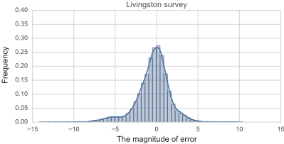
Second, we assumed that the forecast errors by humans are unbiased, that is, the average forecast error is 0, as mentioned in Section 3.1. To verify this assumption, we investigated the error distributions when individuals forecast the annual CPI change rate. Number of samples were 5258 for Livingston Survey and 4706 for SPF. Figure 1 shows the case of Livingston Survey. We omit the figure of SPF due to space constraint. A large portion of forecast values were in the range of [-5, 5] for both surveys. The means of these distributions were -0.40 in the Livingston Survey and 0.37 in the SPF.
| CPI-LIV | CPI-SPF | CoreCPI | PCE | CorePCE | CPI-6M | CPI-1998 | |
|---|---|---|---|---|---|---|---|
| target index | CPI | CPI | CoreCPI | PCE | CorePCE | CPI | CPI |
| survey source | LIV | SPF | SPF | SPF | SPF | LIV | LIV |
| forecast period | 12M | 12M | 12M | 12M | 12M | 6M | 12M |
| boundary | 2008 | 2008 | 2008 | 2008 | 2008 | 2008 | 1998 |
| number of training data | 588 | 564 | 564 | 564 | 564 | 594 | 468 |
| number of test data | 17 | 32 | 32 | 32 | 32 | 17 | 37 |
| ARMA | 1.000 | 1.000 | 1.000 | 1.000 | 1.000 | 1.000 | 1.000 |
| RNN | 0.889 | 0.889 | 0.788 | 0.933 | 0.842 | 1.010 | 0.941 |
| Survey | 0.704 | 0.736 | 0.767 | 0.711 | 0.848 | 0.939 | 0.940 |
| Ensemble | 0.689 | 0.736 | 0.767 | 0.724 | 0.827 | 0.931 | 0.755 |
| var(εh) | 2.869 | 1.887 | 1.379 | 1.453 | 1.134 | 0.986 | 2.952 |
| cov(εh) | 1.846 | 0.873 | 0.455 | 0.450 | 0.168 | 0.652 | 1.924 |
| cov(εθ , εh) | 1.772 | 1.096 | 0.668 | 0.510 | 0.056 | 0.497 | 1.821 |
Upper: Seven datasets and their attributes. LIV stands for Livingston Survey. 6M and 12M stand for 6 months and 12 months, respectively. Middle: Relative RMSEs of each forecasting method in test set. Bold entries are smallest RMSEs in each column. Lower: Parameter values of each dataset estimated from the training set.
Table 1: Forecast accuracy
Based on the observation of the figure, we concluded that the means of the error distributions are close to zero. The numbers of samples are large, i.e., 5258 in the Livingston survey and 4706 in the SPF. Thus, we did not employ the statistical analysis such as t-test for drawing a conclusion.
5.2 Forecast Accuracy
How accurate is the forecast with our human-machine ensemble method? The middle part of Table 1 shows the relative RMSEs for the test set of each forecasting method. Each entry reports the ratio of its RMSE to that of the benchmark, ARMA(1,1). That is, if the value is smaller than 1, it is more accurate than the benchmark; otherwise, it is less accurate than the benchmark.
Our human-machine ensemble method made the most accurate forecasts in four out of the seven datasets, CPI-LIV, CorePCE, CPI-6M, CPI-1998. In two other datasets, CPISPF and CoreCPI, the RMSEs were the same as those from the surveys, and it was the best value among the four methods. This is because the variances outputted by the RNN model were larger than cov(εh) of the SPF, and our ensemble method always selected to use humans only.
We further investigate the behavior of our human-machine ensemble method for CPI-LIV. There were seventeen items (June 2008, December 2008, ..., June 2016) included in the test set. For the fourteen items, no human forecast is incorporated, which means our method succeeded in reducing the expenses for recruiting human forecasters. Among the fourteen items, the maximum squared error was 5.08 in June 2015, and the minimum value was 0.02 in June 2014. However, compared to using the RNN model, our ensemble method could largely reduce the squared error from 11.06 to 6.81 in December 2008, 30.23 to 11.80 in June 2009, and 2.51 to 0.55 in June 2012. That is, when the RNN error is quite large, our ensemble method is effective in reducing the errors.
5.3 Determinant of the Performance of Our Human-machine Ensemble Method
Under what conditions does our human-machine ensemble method perform well? The lower part of Table 1 shows var(εh), cov(εh), and cov(εθ, εh) of each dataset. They were estimated from the training set. The var(εh) is the average variance of the individual errors in a survey; cov(εh) is the average covariance in errors of any human pair; and cov(εθ, εh) is the average covariance in the errors of the RNN model and humans. From the assumptions, the smaller the var(εh), the more accurate the group of humans; the smaller the cov(εh), the more diverse the group of humans; and the smaller the cov(εθ, εh), the more the forecasts of humans and machine differ.
Let us look at cov(εh) and cov(εθ, εh). For CPILIV, CorePCE, CPI-6M, and CPI-1998, where our ensemble method performed well, cov(εθ, εh) was smaller than cov(εh). That is, the forecasts by humans and machines were more diverse than that of only humans. On the other hand, for CPI-SPF, CoreCPI, and PCE, where our ensemble method did not improve the accuracy, cov(εθ, εh) was larger than cov(εh). This means that adding a machine to a group of humans does not increase the diversity of forecasts. We can conclude that performance is determined by the relation between cov(εh) and cov(εθ, εh). If cov(εθ, εh) is larger than cov(εh), our human-machine ensemble method performs well.
5.4 Applicability
When we apply our human-machine ensemble method for other forecasting tasks, a problem is whether the method can have access to an arbitrary number of human experts. Human forecasts collected through crowdsourcing might be able to substitute the surveys of experts such as the Livingston Survey and SPF. Whereas surveys such as the Livingston Survey and SPF employ specific experts, crowdsourcing employs ordinary people. However, the Michigan survey 5 , which is a survey for economic forecasts, employs ordinary people and makes as accurate forecasts as the Livingston Survey and SPF [Ang et al., 2007]. This implies that similar accuracy can be obtained even if crowdsourcing is used for our ensemble method instead of surveys by experts.
5 http://www.sca.isr.umich.edu/
Another problem is how to obtain the parameter values of our human-machine ensemble method. We assumed that the variance of humans' forecasts is known in the theoretical analysis, and estimated the parameter values from the forecasts for the training set in the experiments. Here, we know that performance is explained by the relation between cov(εθ, εh) and cov(εh). This does not directly answer the availability of the variance of humans' forecasts but helps us to determine whether to employ our ensemble method.
6 Conclusion
We proposed a human-machine ensemble method for economic forecasts. Machines and humans make forecasts in different ways. Forecasters based on machine learning techniques perform well if the patterns similar to the input are included in the training data, while humans can take varied information into account and adapt to unforeseen situations. However, traditional ensemble methods cannot use these differences. Therefore, our ensemble method dynamically changes the combination of the machine and humans depending on input.
We conducted an experiment of applying the proposed method to actual inflation forecasts. We created RNN forecast models and combined them with survey data on inflation forecasts and evaluated for seven datasets. The results show that the proposed method improved forecast accuracy for four datasets and achieved the same accuracy as the traditional methods for two datasets.
In this paper, we assume that human forecasters belong to a single type, i.e., the forecast accuracy is defined for a group of human forecasters. Considering more than one types may be possible. For example, experts and non-experts, forecasters of academia and forecasters of the industry. Examining such cases is included in our future work.
Acknowledgments
This research was partially supported by a Grant-in-Aid for Scientific Research (A) (17H00759, 2017-2020) from Japan Society for the Promotion of Science (JSPS).
@inproceedings{ijcai2018p64,
  title     = {Dynamically Forming a Group of Human Forecasters and Machine Forecaster for Forecasting Economic Indicators},
  author    = {Miyoshi, Takahiro and Matsubara, Shigeo},
  booktitle = {Proceedings of the Twenty-Seventh International Joint Conference on
               Artificial Intelligence, {IJCAI-18}},
  publisher = {International Joint Conferences on Artificial Intelligence Organization},
  editor    = {Jérôme Lang},
  pages     = {461--467},
  year      = {2018},
  month     = {7},
  note      = {Main track},
  doi       = {10.24963/ijcai.2018/64},
  url       = {https://doi.org/10.24963/ijcai.2018/64},
}
TY - CPAPER TI - Dynamically Forming a Group of Human Forecasters and Machine Forecaster for Forecasting Economic Indicators AU - Miyoshi, Takahiro AU - Matsubara, Shigeo T2 - Proceedings of the Twenty-Seventh International Joint Conference on Artificial Intelligence, IJCAI-18 PB - International Joint Conferences on Artificial Intelligence Organization PY - 2018 SP - 461 EP - 467 DO - 10.24963/ijcai.2018/64 UR - https://doi.org/10.24963/ijcai.2018/64 ER -Copied
Machine-readable versions of this paper, for tools and AI agents:





