
Stochastic Constraint Propagation for Mining Probabilistic Networks
Proceedings of the Twenty-Eighth International Joint Conference on Artificial Intelligence. Main track. Pages 1137-1145.
https://doi.org/10.24963/ijcai.2019/159
Keywords
- Constraints and SAT: Global Constraints
- Uncertainty in AI: Uncertainty in AI
- Heuristic Search and Game Playing: Combinatorial Search and Optimisation
- Uncertainty in AI: Exact Probabilistic Inference
Abstract
A number of data mining problems on probabilistic networks can be modeled as Stochastic Constraint Optimization and Satisfaction Problems, i.e., problems that involve objectives or constraints with a stochastic component. Earlier methods for solving these problems used Ordered Binary Decision Diagrams (OBDDs) to represent constraints on probability distributions, which were decomposed into sets of smaller constraints and solved by Constraint Programming (CP) or Mixed Integer Programming (MIP) solvers. For the specific case of monotonic distributions, we propose an alternative method: a new propagator for a global OBDD-based constraint. We show that this propagator is (sub-)linear in the size of the OBDD, and maintains domain consistency. We experimentally evaluate the effectiveness of this global constraint in comparison to existing decomposition-based approaches, and show how this propagator can be used in combination with another data mining specific constraint present in CP systems. As test cases we use problems from the data mining literature.
- [Bryant, 1986] Randal E. Bryant. Graph-based algorithms for Boolean function manipulation. IEEE Trans. Comput- ers, 35(8):677-691, 1986.
- [Caseau and Laburthe, 2000] Yves Caseau and Franc ¸ois Laburthe. Solving various weighted matching problems with constraints. Constraints, 5(1/2):141-160, 2000.
- [Charnes and Cooper, 1959] Abraham Charnes and William W. Cooper. Chance-constrained programming. Management Science, 6(1):73-79, 1959.
- [Darwiche, 2001] Adnan Darwiche. On the tractable count- ing of theory models and its application to truth main- tenance and belief revision. Journal of Applied Non- Classical Logics, 11(1-2):11-34, 2001.
- [Darwiche, 2003] Adnan Darwiche. A differential approach to inference in Bayesian networks. J. ACM, 50(3):280- 305, 2003.
- [Darwiche, 2011] Adnan Darwiche. SDD: A new canonical representation of propositional knowledge bases. In IJCAI, pages 819-826. IJCAI/AAAI, 2011. IJCAI
- [De Raedt et al., 2007] Luc De Raedt, Angelika Kimmig, and Hannu Toivonen. ProbLog: A probabilistic Prolog and its application in link discovery. In IJCAI, pages 2462- 2467, 2007. IJCAI
- [De Raedt et al., 2008] Luc De Raedt, Kristian Kersting, An- gelika Kimmig, Kate Revoredo, and Hannu Toivonen. Compressing probabilistic Prolog programs. Machine Learning, 70(2-3):151-168, 2008.
- DTAI Research Group, KU Leuven, 2015 2019] DTAI Re- search Group, KU Leuven. ProbLog Python library. https: //bitbucket.org/problog/problog, 2015-2019. Link
- [Dueñas-Osorio et al., 2017] Leonardo Dueñas-Osorio, Kuldeep S. Meel, Roger Paredes, and Moshe Y. Vardi. Counting-based reliability estimation for power- transmission grids. In AAAI, pages 4488-4494, 2017.
- [Fierens et al., 2015] Daan Fierens, Guy Van den Broeck, Joris Renkens, Dimitar Shterionov, Bernd Gutmann, Ingo Thon, Gerda Janssens, and Luc De Raedt. Inference and learning in probabilistic logic programs using weighted Boolean formulas. TPLP, 15(3):358-401, 2015.
- [Gange et al., 2010] Graeme Gange, Peter J. Stuckey, and Vitaly Lagoon. Fast set bounds propagation using a BDD- SAT hybrid. J. Artif. Intell. Res., 38:307-338, 2010.
- [Hawkins and Stuckey, 2006] Peter Hawkins and Peter J. Stuckey. A hybrid BDD and SAT finite domain constraint solver. In PADL, volume 3819 of Lecture Notes in Com- puter Science, pages 103-117. Springer, 2006.
- [Hemmi et al., 2018] David Hemmi, Guido Tack, and Mark Wallace. A recursive scenario decomposition algorithm for combinatorial multistage stochastic optimisation prob- lems. In AAAI, pages 1322-1329, 2018.
- [Kempe et al., 2003] David Kempe, Jon M. Kleinberg, and Éva Tardos. Maximizing the spread of influence through a social network. In KDD, pages 137-146. ACM, 2003.
- [Latour et al., 2017] Anna L. D. Latour, Behrouz Babaki, Anton Dries, Angelika Kimmig, Guy Van den Broeck, and Siegfried Nijssen. Combining stochastic constraint opti- mization and probabilistic programming -from knowledge compilation to constraint solving. In CP, volume 10416 of Lecture Notes in Computer Science, pages 495-511. Springer, 2017.
- [Littman et al., 1998] Michael L. Littman, Judy Goldsmith, and Martin Mundhenk. The computational complexity of probabilistic planning. J. Artif. Intell. Res., 9:1-36, 1998.
- [Newman, 2001] Mark E.J. Newman. The Structure of Sci- entific Collaboration Networks. Proceedings of the Na- tional Academy of Sciences, 98(2):404-409, 2001.
- [OscaR Team, 2012] OscaR Team. OscaR: Scala in OR, 2012. Available from https://bitbucket.org/oscarlib/oscar. Link
- [Ourfali et al., 2007] Oved Ourfali, Tomer Shlomi, Trey Ideker, Eytan Ruppin, and Roded Sharan. SPINE: A framework for signaling-regulatory pathway inference from cause-effect experiments. In ISMB/ECCB (Supple- ment of Bioinformatics), pages 359-366, 2007.
- [Perez and Régin, 2017] Guillaume Perez and Jean-Charles Régin. MDDs: Sampling and probability constraints. In CP, volume 10416 of Lecture Notes in Computer Science, pages 226-242. Springer, 2017.
- [Pipatsrisawat and Darwiche, 2009] Knot Pipatsrisawat and Adnan Darwiche. A new d-DNNF-based bound computa- tion algorithm for functional E-MAJSAT. In IJCAI, pages 590-595, 2009.
- [Rossi et al., 2006] Francesca Rossi, Peter van Beek, and Toby Walsh, editors. Handbook of Constraint Program- ming, volume 2 of Foundations of Artificial Intelligence. Elsevier, 2006.
- [Roth, 1996] Dan Roth. On the hardness of approximate rea- soning. Artif. Intell., 82(1-2):273-302, 1996.
- [Schaus et al., 2017] Pierre Schaus, John O. R. Aoga, and Tias Guns. Coversize: A global constraint for frequency- based itemset mining. In CP, volume 10416 of Lec- ture Notes in Computer Science, pages 529-546. Springer, 2017.
- [Tarim et al., 2009] S. Armagan Tarim, Brahim Hnich, Steven David Prestwich, and Roberto Rossi. Finding re- liable solutions: event-driven probabilistic constraint pro- gramming. Annals OR, 171(1):77-99, 2009.
- [Verhaeghe et al., 2018] Hélène Verhaeghe, Christophe Lecoutre, and Pierre Schaus. Compact-MDD: Efficiently filtering (s)MDD constraints with reversible sparse bit-sets. In IJCAI, pages 1383-1389, 2018. IJCAI
- [Walsh, 2002] Toby Walsh. Stochastic constraint program- ming. In ECAI, pages 111-115. IOS Press, 2002. IJCAI
- [Xue et al., 2017] Yexiang Xue, XiaoJian Wu, Dana Morin, Bistra Dilkina, Angela Fuller, J. Andrew Royle, and Carla P. Gomes. Dynamic optimization of landscape connectivity embedding spatial-capture-recapture infor- mation. In AAAI, pages 4552-4558. AAAI Press, 2017.
References were extracted automatically from the PDF and may contain errors.
Full text extracted automatically from the PDF; figures, tables and equations may differ. The PDF is the version of record.
1 Introduction
Making decisions under uncertainty is an important problem in business, governance and science. Examples are found in the fields of planning and scheduling, but also occur naturally in fields like data mining and bioinformatics.
Consider for example a viral marketing problem, as studied in the data mining literature [Kempe et al., 2003]. We are given a social network of people (vertices) that have stochastic relationships (edges). We want to rely on word-of-mouth advertisement to turn acquaintances of people who buy our product into new product-buyers. How can we find the k most influential nodes in this social network?
Or consider the problem of signaling-regulatory pathway inference [De Raedt et al., 2008; Ourfali et al., 2007]. We are given a network of probabilistic protein-gene interactions (edges). We are also given (protein, gene) pairs representing relationships of interest to a particular biologist. How can we select a small subset of edges from the network to provide insight in how the (protein, gene) pairs relate to each other?
Myriad variations of these problems exist. Consider this variation of influence spreading in citation networks: next to the network, we are given a database of papers and their authors. How can we enumerate all sets of authors that coauthored many papers, and that had a minimum level of influence in the network? Here, we extend the viral marketing problem with an extra requirement formalized over a second database, and no longer solve an optimization problem.
We observe that these problems are instances of a general class of problems, which we call stochastic constraint optimization or satisfaction problems on monotonic distributions (SCPMD). These constraint satisfaction or optimization problems have the following characteristics: (1) they can be formulated on probabilistic networks and involve the calculation of a probability or an expectation on such networks; (2) the probabilities and expectations are higher if more nodes or edges are selected; (3) constraints limit these selections. While characteristic (2) seems limiting, problems with this characteristic are plentyful. Examples include the two applications mentioned above, but also an optimisation variant of the network reliability [Due˜nas-Osorio et al., 2017] and a variant on landscape connectivity [Xue et al., 2017]. Section 7 discusses the relation of SCPMDs to other problems.
In this work we develop a generic approach for solving such SCPMDs. SCPMDs are not easy to solve. The calculation of a probability in probabilistic networks requires solving a counting problem. This counting problem is known to be hard (#P complete) [Roth, 1996]; well-known instances of SCPMDs, such as spread-of-influence problems, are NPhard [Kempe et al., 2003]. Overall, SCPMDs require solving both constraint satisfaction and counting problems.
There is limited earlier work on solving SCPMDs. Our work continues the line of our earlier work ([Latour et al., 2017]), which proposed to solve SCPMDs as follows: (1) a probabilistic programming language, SC-ProbLog, was introduced to model these problems; this language extends a probabilistic logic programming language, ProbLog [De Raedt et al., 2007], that has often been used in the literature to model distributions over networks; (2) statements in this language are used to compile decision diagrams, either Ordered Binary Decision Diagrams (OBDDs) or Sentential Decision Diagrams (SDDs), that represent the distributions; (3) the diagrams are decomposed to create inputs for existing generic solvers: either Constraint Programming (CP) or Mixed Integer linear Programming (MIP) solvers.
Our main contributions in this work are the following. We show that the earlier CP decomposition approach is not generalized arc consistent (GAC), and that a straightforward arc consistent modification of this earlier approach does not perform well. To solve this, we introduce a constraint propagation algorithm for a global constraint on OBDD representations of monotonic distributions, which we call the Stochastic Constraint on Monotonic Distributions (SCMD), and we demonstrate the benefits of this global constraint.
In summary, the benefits of our global constraint are: (1) it guarantees generalized arc consistent (GAC), contrary to the decomposition method described above (Section 4); (2) it has a worst-case complexity of O(m + n) with OBDD size m and n decision variables (Section 5); (3) it outperforms existing CP-based methods and complements MIP-based methods, while scaling better with OBDD size than MIP-based methods (Section 6); as a result, the costly process of OBDD or SDD minimization is less important using our constraint; and (4) it supports modeling a larger range of SCPMDs than MIP-based methods can (e.g., enumeration problems).
Note that a number of approaches in the literature are not related to this work. We do not use OBDDs as a compact representation for satisfying assignments to a global constraint; we use them as a representation of a probability distribution (Sections 3, 5 and 7), which means that we are not able to build on existing propagators for OBDDs. Note also that we do not solve problems that can be solved using maxSAT solvers, since maxSAT has no concept of counting (Section 3), which we require to solve SCPMD problems.
2 Modeling SCPMDs
We consider constraint satisfaction and optimization problems that are defined on Boolean decision variables. We are interested in finding one or more assignments to these decision variables, such that given constraints are satisfied, and, if provided, an optimization criterion is optimized. We also refer to such assignments as strategies. The specific feature of stochastic constraint satisfaction problems is that the constraints, as well as the optimization criterion, may be stochastic and require some form of counting.
The stochastic constraint studied in this work is this:
The sum represents an expected utility, in which Φ is a set of stochastic events, P (φ | σ) represents the probability of an event φ happening, given a strategy σ; ρφ ∈ R+ is a reward for this event. For simplicity we will assume ρφ = 1 in this work. Note that generalizing our approach to ρφ ̸= 1 is trivial: in only involves multiplying conditional probabilities with the appropriate reward before summing and comparing to threshold θ ∈ R+.
In SCPMDs, we require each probability P (φ | σ) to be monotonic: for any strategy σ, switching the value of any decision variable from false to true, will yield a probability that is not smaller: P (φ | σ′ ) ≥ P (φ | σ), if σ′ differs from σ by one variable that is true in σ′ but false in σ. This condition is
Figure 1: A network of four nodes (a, b, c and e) and four undirected edges with mutually independent probabilities.
met in the example problems mentioned earlier. We will refer to our constraint as a Stochastic Constraint on Monotonic Distributions (SCMD).
Our results are straightforwardly expanded towards maximization problems over expected utilities.
Example 2.1 (Viral Marketing: SCPMD). Problems on networks, e.g. viral marketing problems, can be seen as SCPMDs such as defined earlier. Consider the network in Figure 1. Suppose that the edges represent probabilistic mutual trust relationships, meaning that individuals u and v trust each other with the probability puv that is the label on edge (u, v), and do not trust each other with probability (1 - puv).
For the sake of this example, we make the following simplifying assumptions: (1) once someone gets a free product sample, they will certainly buy the product; (2) if a trusted friend buys the product, they will also buy the product. The problem is to maximize the expected number of people buying our product, given a limited number k of free samples to distribute to people in the network.
We model this as follows:
- with each node i in the network we associate a Boolean decision variable di, representing if person i gets a free sample;
- the events considered are φa, φb, φc and φe, where φi expresses the event of person i buying our product;
- our objective is to find a strategy σ that maximizes the expected utility ∑i∈{a,b,c,e} P (φi | σ);
- constraint: ∑i∈{a,b,c,e} di ≤ k (threshold k ∈ N+).
Note that in this example, we have a stochastic objective function rather than a stochastic constraint, like the one in Equation (1). However: we can maximise the expected utility by solving ∑i∈{a,b,c,e} P (φi | σ) > θ, increasing θ to the best expected utility for a solution found so far, each time we find such a solution, until no new solution can be found.
We also need to define the probability of events φi, given a strategy. While there are many formalisms for defining these conditional probabilities, we use a Weighted Model Counting (WMC) approach in this work, where weighted propositional formulas define the distributions; this approach generalizes many other well-known approaches.
Example 2.2 (Viral Marketing: WMC). The situations in which the event φe is considered to take place are defined by the propositional formula φe = de ∨ (dc ∧ tcd) ∨ (db ∧ tbc ∧ dce) ∨ (da ∧ tac ∧ dce) ∨ (db ∧ tba ∧ tbc ∧ dce) ∨ (da ∧ tab ∧ tbc ∧ dce). The logical formula represents all the different situations in which e will finally buy the product. We use two types of variables: (1) the di variables are the decision variables of the SCPMD; (2) the tij variables are associated to each edge (i, j) in the network and represent trust. In our example, one possibility for event φd to happen is when person c gets a free sample and person e trusts person c.
To define a distribution over the network, we associate a probability p (tij) with each Boolean variable tij that this variable is true. We call tij a stochastic variable. The probability P (φe | σ) is then defined as the sum of the probabilities of all the (logical) models of this formula, given the strategy. Given strategy σ = (da = ⊤, db = dc = de = ⊥), one model is for instance tac = tce = ⊤, tab = tbc = ⊥, of which the probability is 0.8 · 0.3 · (1 - 0.4) · (1 - 0.1) = 0.1296.
Ensuring that distributions are monotonic is relatively easy in the WMC approach: if our logic formula is equivalent to a formula without negation, the distribution defined by it is monotonic. There are various methods for obtaining propositional formulas like φe. We use ProbLog [De Raedt et al., 2007; Fierens et al., 2015].
3 Solving SCPMDs
We discuss briefly how OBDDs [Bryant, 1986] have been used to solve SCPMDs in earlier work. OBDDs are compact representations for the satisfying assignments of a constraint. While this property was used for constraint propagation before [Gange et al., 2010; Hawkins and Stuckey, 2006], we employ OBDDs differently. We compile formulas such as the one in Example 2.2 to OBDDs to perform weighted model counting (WMC). While compilation and minimization of OBDDs is time-consuming, it allows for more tractable inference afterwards. Other types of diagrams, such as Sentential Decision Diagrams (SDDs) [Darwiche, 2011], can also be used for model counting. While these representations may be smaller, the compilation procedure can be time consuming. We will show experimentally that compiling smaller diagrams may not always yield better overall running times.
To see how we can compute P (φ | σ) using an OBDD, consider Figure 2. It shows an OBDD that represents the probability of the formula in Example 2 evaluating to true. The weights on the outgoing arcs of nodes that represent stochastic variables (those labeled with tij) correspond to the probability that that variable is true (for the solid, or hi, arcs) or false (dashed, or lo, arcs). A strategy σ is projected on the OBDD by adding weights of 0 and 1 to the outgoing arcs of the nodes labeled with decision variables. For example: if we choose da = ⊥, we label the outgoing hi arcs of nodes labeled with da with 0, and their outgoing lo arcs with 1.
Given a strategy σ and arcs labeled accordingly, the OBDD can straightforwardly be mapped to an Arithmetic Circuit (AC). We can compute P(φe | σ) as follows. In a bottomup traversal, each OBDD node r takes the value
where 0 ≤ w(r) ≤ 1 represents the weight of the variable that labels r, r+ (r-) is the hi (lo) child of r, i.e., the child connected through the solid (dashed) outgoing arc of r; v(r) = 0 for the negative leaf and v(r) = 1 for the positive leaf. Observe that v(root) = P (φ | σ).
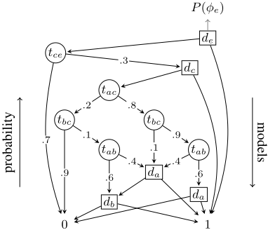
The complexity of evaluating P(φ | σ) is thus linear in the size of the OBDD, but the number of strategies is 2n , with n the number of decision variables. A na¨ıve way of solving a SCPMD that involves enumerating all possible strategies and evaluating their quality using the OBDD does not scale well.
Since SCPMDs are constraint optimization problems, one obvious approach to improving on the enumeration method is to leverage existing CP solvers. The tool chain described in our earlier work [Latour et al., 2017] decomposes an OBDD into a set of linear constraints that can be put into a MIP solver or CP solver; auxiliary variables represent the value at each node of the OBDD according to Equation (2).
4 CP, Decomposition and GAC
We recall a few basic concepts of CP. A comprehensive overview can be found in the literature [Rossi et al., 2006].
4.1 Seach, Propagation, Consistency
Discrete optimization problems in CP are modeled using a set of variables X = {x1, . . . , xn}, each of which is associated with a domain dom(xi) ⊆ D (with D = {a1, . . . , ad} a set of values), a set of constraints on the variables C and an objective function f(X).
CP solvers use a depth-first traversal through a search tree to find an optimal solution. The solver repeatedly selects an unbound variable x and assigns to it a value a ∈ dom(x) (or a range or interval of values in case, e.g., dom(x) ⊆ R), thus building a partial solution. Selecting an unbound variable and assigning a value to it is called branching.
After each time the solver branches, propagation updates the domains of the remaining unbound variables by removing values that would violate the constraints of the problem, given the current partial solution. If the size of a variable x's domain is reduced to 1 in this process, we consider x fixed to the remaining value in dom(x). If for any variable x we find
|dom(x)| = 0, we have encountered a failure: a partial assignment that cannot be extended to a solution. A (variable, value) pair (x, a) with a ∈ dom(x) is considered Generalized Arc Consistent (GAC) with respect to a constraint c ∈ C iff there exists an assignment in which x = a, that satisfies c.
In general, variables have different kinds of domains (discrete, categorical, continuous, etcetera). The propagation algorithm we present in this work operates on constraints that involve only Boolean decision variables.
4.2 GACGuarantees of Decomposition
Unfortunately, our earlier approach, that decomposes the OBDD into a set of linear constraints [Latour et al., 2017], is not GAC:
Theorem 4.1. Propagation on the decomposed representation of the Stochastic Constraint on Monotonic Distributions as described in [Latour et al., 2017] is not GAC.
Proof. Let us assume that propagation in the decomposition method from [Latour et al., 2017] would be GAC. Then, the following counter example leads to a contradiciton.
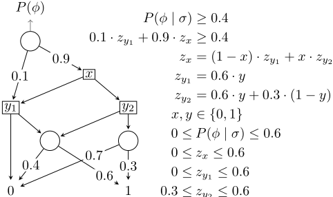
Consider the OBDD in Figure 3 and the associated constraint P(φ | σ) ≥ 0.4. Observe that the four possible strategies yield the following conditional probabilities:
From this we conclude that only those strategies in which y = 1 holds, can possibly satisfy the constraint. A propagator that ensures GAC on the Boolean variables will detect this before the start of the search and fix y to 1.
The circuit decomposition method uses Equation (2) to translate this constraint on the OBDD in a CP model, which is also given in Figure 3. Note that this model introduces auxiliary variables z with domains that include real numbers.
Suppose a propagator is called on this decomposed model, before the search starts. This propagator may start by trying to infer the minimum value that zy1 needs to take if zx takes its maximum possible value. To do this, the propagator assumes that zx = 0.6 holds. Now it can infer that, in order for the constraint to be satisfied, zy1 ≥ (0.4 - 0.9 · 0.6)/0.1 = -1.4 should hold. Unfortunately, it already knew that dom(y) = {0, 1} and thus does not include -1.4. Based on this, it cannot remove 0 from dom(y). Repeating a similar procedure to determine a bound for zx, zy1 and zy2 does not yield conclusive evidence to deduce that y must be fixed to 1, either.
As a result, the search tree of a CP system is unnecessarily large. One solution may seem to create a decomposed representation that is GAC. We can do this by making two modifications to the decomposition method. First, we replace the encoding of the value of OBDD node rd,
with v(rd) = max (d · v(r+ d ), (1 - d) · v(rd )), because this improves propagation in cases where d is yet unassigned.
Additionally, we add the (redundant) constraint v|d=0(root) < θ → d = 1 to the decomposition for each decision variable d. Here, v|d=0(root) represents the expression at the root of the diagram as obtained with Equation (2), conditioned on d = ⊥. The downside of this approach is that we need to add a large number of linear constraints to the model, resulting in a space complexity of this approach of O(|X| · |OBDD| · τ), with X the set of decision variables, |OBDD| the size of the OBDD and τ the depth of the search tree. We demonstrate the practical inferiority of this approach in Section 6.
5 Approach
We intend to improve upon the existing approach by allowing an OBDD-based SCMD to be added directly to a CP solver as a global constraint. We first define the SCMD and then introduce a propagator for OBDDs that guarantees GAC.
5.1 Stochastic Constraint onMonotonic Distributions
We define a monotonic distribution as follows:
Definition 5.1. Let φ(X, T) be a propositional formula on Boolean decision variables X and Boolean stochastic variables T. Let P(φ | σ) be the probability that φ evaluates to ⊤, given strategy σ that assigns truth values to decision variables d ∈ X. We call the probability distribution P(φ | σ) a monotonic distribution if there exists an OBDD for φ, whose score at the root equals P(φ | σ) and for which the following property holds for any projected σ (see Section 3):
for each OBDD node rd that is labeled with decision variable d ∈ X, where v() is computed using Equation (2).
We now define a corresponding SCMD as follows:
Definition 5.2. For a set of propositional formulas Φ on Boolean decision variables X and Boolean stochastic variables T, threshold θ ∈ R+ and utilities ρφ ∈ R+, we call
a Stochastic Constraint on Monotonic Distributions (SCMD) if all P(φ | σ) are monotonic distributions.
Given a partial strategy σ, a GAC-guaranteeing propagator for the SCMD will, for each unbound decision variable d ∈ X, remove the value ⊥ from dom(d) if
holds for each possible extension of σ to a full strategy σ′ that includes d = ⊥.
5.2 Na¨ıve (Quadratic) OBDD Propagation
For maintaining GAC, a key observation is that our scoring function (the expected utility in Equation (4)) is monotonic; hence, the largest possible score is obtained by assigning the value true to all unbound decision variables. The following process for each unbound decision variable d would be GAC: (1) fix variable d to the value false; (2) fix all remaining unbound variables to the value true; (3) calculate the score for the resulting assignment; (4) if the score is lower than the desired threshold, remove the value false from dom(d).
The score calculated in step 3 is an upper bound for the value of the OBDD, given the current partial assignment and that d = ⊥. Note that this algorithm does not require us to put constraints on the variable order of the OBDD to obtain the strict bound in step 3, contrary to previous work using SDDs and d-DNNFs [Pipatsrisawat and Darwiche, 2009].
Let n be the number of unbound decision variables, and let m be the size of the OBDD. Then the complexity of this na¨ıve OBDD propagator is O(mn): for every unbound variable we perform a bottom-up traversal of the OBDD. Since propagation is the most computationally intensive part of search algorithms under our constraint, it is important to obtain a better performance. We will improve this complexity to O(n+m).
5.3 Linear OBDD Propagation
The key idea behind improving the propagator is that we calculate a derivative ∂f(d,σ′ \d) ∂d = f (σ′ ) - f (d = ⊥, σ′ \ d) for every unbound decision variable d; σ′ represents an assignment to all decision variables obtained by taking a partial assignment σ and assigning true to each unbound variable in σ. Function f represents the function defined by Equation (2) on the root of the OBDD.
We use the derivative to remove the value false from the domains of variables that do not meet the following condition:
The main question becomes how to calculate the partial derivative for all unbound variables efficiently. Here, we build on ideas introduced by Darwiche [Darwiche, 2001; Darwiche, 2003] to build a linear algorithm that can furthermore maintain derivatives incrementally. We first need to define the concept of path weight:
Definition 5.3. Let rm be a node labeled with variable xm in an OBDD with variable order x1 < . . . < xn. We define the path weight of rm:
where ℓ is a path from the root of the OBDD to rm, and Lrm is the set of all such paths that are valid. A path is valid if it does not include the hi (lo) arc from a node labeled with a decision variable that is false (true or unbound).
We define u(i) as follows. For the outgoing arcs of decision nodes that can be part of a valid path, we use u(i) = 1. For the outgoing arcs of stochastic nodes labeled with a stochastic variable xi that has weight w(i), we use:
The path weight π(rm) is expressed in terms of variables xi < xm only.
Our algorithm is based on the following observation:
Theorem 5.1. The derivative of the OBDD with respect to a decision variable can be calculated as follows:
with OBDDd the set of OBDD nodes labeled with variable d.
To prove the theorem, we simply write down an expression for f(x1, . . . , xm, . . . , xn) (with x1 ≤ xm ≤ xn in the variable order) using Equation (2). Then we rearrange the terms according to variable order such that they can be separated in an expression for the path weight π(rm) for a node rm and its value. Finally, we take the partial derivative, and show that this equals Equation (9).
We use the observation above to create an O(m) algorithm for calculating all derivatives in two stages: (1) a topdown pass over the complete OBDD for calculating all path weights; (2) a bottom-up pass for calculating the values for all nodes in the complete OBDD, calculating the derivatives for each variable in the process.
The top-down pass operates as follows. We initialize the path weight π(r) of each node with 0. We update the path weight of its children r+ and r- as follows if r is labeled with a decision variable d:
If r is labeled with a stochastic variable with weight w, we assign π (r+) + wπ(r) to π (r+) and π (r-) + (1 - w) π(r) to π (r-).
We compute the node values in a bottom-up pass, using Equation (2) with w(r) = 0 if r corresponds to a decision variable that is false, and w(r) = 1 otherwise.
During this bottom-up pass, we can recompute the derivatives for all decision variables that are still unbound using Equation (9), and evaluate Equation (6) for each of those to see if we can remove false from their domain.
Clearly, the overall calculation finishes in O(n+m) time.
5.4 Sub-linear OBDD Propagation
We can reduce the complexity of the algorithm above further by avoiding the traversal of unnecessary parts of the OBDD. These observations allow for more efficient propagation:
- (O1) As noted before, the expression for the path weight of an OBDD node labeled with variable xm (Equation (7)) only contains variables xi < xm. We conclude that fixing a decision variable d can only affect the path weights of nodes below the nodes labeled with that variable d.
- (O2) Path weights below unbound decision nodes are not changed when we fix an unbound decision node to true. Therefore: our propagator only needs to update path weights if we fix a decision variable to false.
- (O3) Similarly, fixing a variable can only affect the values of the nodes labeled with that variable themselves, and those above them in the OBDD. Again: only fixing a variable to false requires the propagator to update values.
- (O4) We do not need to maintain the values for any of the nodes in the OBDD above the decision nodes closest to the root, as we will never need to calculate the derivative for any variable in that part of the diagram.
- (O5) Similarly, we do not need to maintain path weights for the descendants of the variable closest to the leaves.
- It can be shown that by only maintaining the part of the OBDD between two borders of unbound decision variables (the active part of the OBDD), one can calculate the derivatives exactly, as well as calculate the value of the solution.
- (O6) Some parts of the OBDD will no longer be connected to the root as a consequence of partial assignments. We thus do not need to update those parts of the OBDD.
- (O7) Derivatives can be used in variable branching heuristics to guide our search, as can (O4) and (O5). If we always branch on the variable with the largest derivative, we are likely to find failing partial strategies quickly. By branching on the highest or lowest decision variable, we reduce the size of the active part of the OBDD.
We improve the two-sweep linear OBDD propagation algorithm by addressing these observations. (O1-3) are easily addressed by implementing queues and smartly initializing and updating them such that we start traversing the OBDD downwards (upwards) at the places where path weights (values) may change due to decision variable assignments.
We maintain for each OBDD node r three counters. The first indicates if there is a path from an unbound node above r to r. If there are no such paths, there is no need to update values of nodes above r if the value of r changes (O4). The second indicates if there is a path from r to an unbound node below r. If not, any changes in r's path weight need not be propagated down from r (O5). The third indicates if there is a valid path from the root to r. If not, r's path weight is 0, and changes in its value need not propagate (O6). Maintaining these counters requires two extra passes through the OBDD each time the propagator is called. But: they allow us to traverse an ever decreasing part of the OBDD in each pass.
| name | |OBDD| | |OBDDmin| | tmin[s] | Nt | Nd |
|---|---|---|---|---|---|
| hep-th47 | 10, 815 | 6, 504 | 901 | 51 | 20 |
| hep-th5 | 52, 009 | 4, 708 | 7, 357 | 90 | 33 |
| spine27a | 1, 898 | 1, 898 | 78 | 60 | 60 |
| spine27b | 9, 350 | 9, 322 | 474 | 55 | 55 |
| spine16 | 80 | 80 | 0.86 | 33 | 33 |
Finally, we address (O7) by implementing different variable branching heuristics: top, which always branches on the unbound variable highest in the OBDD, and its counterpart bottom. Each can be combined with a value branching heuristics: either branch first on value 0, or on value 1. We also implement two regret-based [Caseau and Laburthe, 2000] branching heuristics that use the calculated derivatives: derivative1 and derivative0. The former (latter) selects the unbound decision variable with the largest (smallest) absolute derivative and first branches on 1 (0).
Observe that, compared to the GAC-guaranteeing decomposition method described in Section 4.2, the space complexity of this approach is only O(|OBDD| · τ).
6 Experiments
We evaluate the performances of the linear and sub-linear OBDD propagation algorithms (Sections 5.3 and 5.4).
Questions. Our experiments are guided by these questions:
- (Q1) How do solving times depend on the CP encoding of the constraint (decomposed versus global)?
- (Q2) How do branching heuristics affect solving times for the global encoding?
- (Q3) How do solving times for our global constraint for a CP solver compare to those of a decomposed constraint solved with a MIP solver?
- (Q4) How does our propagator's performance depend on OBDD size?
- (Q5) How does our propagator perform when other constraints are added?
6.1 Experimental setup
The implementations of our propagation algorithms and all the code for reproducing our experiments, are available at github.com/latower/SCMD.
Test Data. Since we aim to improve on the performance of our earlier decomposition-based approach [Latour et al., 2017], we evaluate our methods on datasets used in this earlier work: DNA-protein interaction networks spine16, spine27a, spine27b [Ourfali et al., 2007] and collaboration networks datasets hep-th47 and hep-th5 [Kempe et al., 2003; Newman, 2001]. 1 We refer the reader there for a description. Dataset characteristics are given in Table 1.
1 The dataset spine27a in this work corresponds to spine27 in [Latour et al., 2017]. spine27b is a problem on the same network, but optimizing over a different function.
ConstraintOptimizationSetting. Our OBDDpropagators support the optimization task of maximizing an expectation. This is combined with a linear constraint that enforces an upper bound k on the number of decision variables that can be set to true (the cardinality of the solution) in our experiments.
Software. We implemented the OBDD propagators proposed in Sections 5.3 and 5.4 in the Scala 2.12 library OscaR 4.0.0 [OscaR Team, 2012], because we need the state-of-the-art CoverSize 1.0.0 constraint [Schaus et al., 2017] for itemset mining to answer (Q5). 2 We use CP solver Gecode 6.0.1 and MIP solver Gurobi 8.0.0 for comparison experiments. 3 Since OscaR does not support floating point variables, we could not implement the decomposition methods in OscaR. Instead, we implemented them in award-winning Gecode, believing it to be a fair choice for comparison. For modeling we use a SC-ProbLog version based on ProbLog 2.1 [DTAI Research Group, KU Leuven, 2015 2019], running in Python 3.6. 4 We use the dd 0.5.4 library for the OBDD compilation. 5
Configuration. Unless indicated otherwise, we use the default settings for all software. In our experiments to answer (Q1), we constrain both CP solvers to branch on the variables in lexicographical order. For the other experiments, our propagator uses the branching heuristic derivative1 (Section 5.4).
Hardware. Our experiments ran on a machine with eight Xeon E5540 processors and 24GB RAM, under CentOS Linux 7.4.1708. Our results are averaged over two runs, to account for small variations in hardware performance. OBDD minimization times are averaged over five runs instead of two.
6.2 Results
In addition to the results presented here, more experimental results are available at github.com/latower/SCMD.
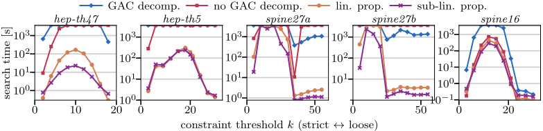
We address (Q1) by comparing the solver search times of the implementations of the linear and sub-linear versions of our propagator with two decomposed approaches in Gecode: one from [Latour et al., 2017] that does not guarantee GAC and the one described in Section 4.2 that does. We keep the branching order for the search process fixed to a lexicographical one. The constraint threshold k indicates the maximum allowed cardinality of the solution: from small (strict) to large (loose). Figure 4a shows that the global OBDD propagator outperforms both decomposition methods on these testcases. While the sub-linear version of our propagator outperforms the linear one, this difference is less pronounced.
We answer (Q2) by evaluating the performance of the branching heuristics described in Section 5.4. In an experiment on the four settings from [Latour et al., 2017], the average runtimes for the different heuristics were as follows. top0: 194s, top1: 1, 030s, bottom0: 233s, bottom1: 229s, derivative0: 1, 206s and derivative1: 87s. Both top1 and derivative0 had one instance timeout after 1 hour, which is the time that is included in these averages.
2 Available at sites.uclouvain.be/cp4dm/fim.
3 Available at www.gecode.org and www.gurobi.com.
4 Available at bitbucket.org/problog/problog/src/sc-problog.
5 Available at pypi.org/project/dd/.
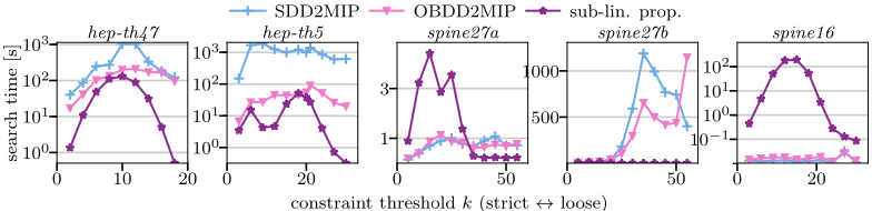
Figure 4b compares the performance of our sub-linear OBDD propagator to two methods that use MIP solver Gurobi for solving the problem. One takes the same OBDD as input as our propagator and decomposes it to a MIP. The other is one of our methods from [Latour et al., 2017], which takes an SDD as input and decomposes that to a MIP. The figure shows that the OBDD-based methods outperform SDDbased methods. We also observe that our propagator outperforms the OBDD-to-MIP method on the more difficult test cases, answering (Q3). We conclude that the CP based and MIP based approaches are complementary in these tasks, CP scaling better in the more time consuming cases.
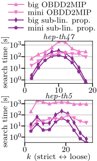
An important aspect in the creation of OBDDs is whether or not to minimize their size. As stated in Section 3, minimization is time-consuming. Our propagator provides the same level of consistency independent of the shape of the circuit. In Figure 4c we compare search time on minimized and big (unminimized) OBDDs. The time necessary for OBDD minimization for hep-th47 is 901s, and 7, 357s for hep-th5 (averages over five runs). Size reductions are about 60% and 90%, respectively. We see that our propagator's performance scales indeed (sub-)linearly with OBDD sizes, answering (Q4), while the decomposed approach's solving times increase more rapidly. Hence, a pipeline that builds an unminimized OBDD and searches using our propagator can be more efficient than alternative MIP pipelines that either use an unminimized OBDD or perform OBDD minimization. In this experiment Gurobi uses eight threads while the sub-linear OBDD propagator uses only one. The lack of scaling of the OBDD-to-MIP approach is even more pronounced when the solvers are compared on the same number of threads.
To answer (Q5), we ran experiments on the enumeration setting described in Section 1, succesfully demonstrating the applicability of our constraint propagator on Itemset Enumeration problems, which were shown to be solved efficiently by CP [Schaus et al., 2017]. We are given a citation network and a database with sets of co-authors. The problem is to find all sets of co-authors that have collaborated at least k times and who have influenced a minimum expected number of other authors by being cited. For a citation network of the International Conference on Inductive Logic Programming, examples of such sets are {Luc De Raedt} and {Ganesh Ramakrishnan, Ashwin Srinivasan}.
7 RelatedWork
SCPMDs are related to chance constraint optimization [Charnes and Cooper, 1959], probabilistic CP [Tarim et al., 2009], stochastic constraint satisfaction problems (SCSPs) [Walsh, 2002] and functional E-MAJSAT [Littman et al., 1998; Pipatsrisawat and Darwiche, 2009].
The main difference between SCPMDs and these problems is that SCPMDs are defined on monotonic distributions. We exploit this property to optimize the constraint propagation process for SCMDs, distinguishing our method from more general approaches taken earlier [Walsh, 2002]. While our propagator can only be applied to monotonic distributions, it does allow us to obtain strict bounds during constraint propagation. These strict bounds can only be achieved in alterconstraint threshold k (strict ↔ loose)
constraint threshold k (strict ↔ loose)
k (strict ↔ loose)
(c) MIP-based decomposition method and sub-linear global OBDD propagation algorithm (with branching heuristic derivative1) on big (not minimized) and mini (minimized) OBDDs.
Figure 4: Experimental results. Timeout in all experiments is 1 hour. 'GAC decomp.' is the GAC-guaranteeing decomposition method (Section 4.2), 'no GAC decomp.' is the decomposition method from [Latour et al., 2017], both are implemented in Gecode. 'lin. prop.' and 'sub-lin. prop.' are the linear and sub-linear OBDD propagation algorithms from Sections 5.3 and 5.4, respectively. 'SDD2MIP' and 'OBDD2MIP' are implementations from [Latour et al., 2017] that convert an SDD and OBDD into a MIP, solving it with Gurobi.
native methods [Pipatsrisawat and Darwiche, 2009] by constraining the underlying variable order of the decision diagrams. The variable order of a diagram determines its size, and the efficiency of constraint propagators depends on the size of the diagrams they are operating on. Therefore, having extra constraints on the variable order that limit possibilities of obtaining a sufficiently small diagram, is disadvantageous.
Our approach of keeping (global) constraints (such as a linear constraint on cardinality) separated has the advantage that it avoids the complexity of encoding this combination of constraints in one diagram, if we were to follow the approach of [Pipatsrisawat and Darwiche, 2009]. Consequently, we avoid the blow-up of the diagram, we exploit the structure of these constraints and thus leverage the power of dedicated constraint solvers. Finally, modeling constraints separately allows the user to add constraints that cannot be (trivially) encoded in CNF. This allows for larger expressiveness than the method in [Pipatsrisawat and Darwiche, 2009].
The main feature that distinguishes our work from similar works on stochastic constraint satisfaction and optimization is that we exploit the structure of the probability distribution in our solving method. The majority of existing methods sample scenarios from a distribution, and hence ignore such structures [Hemmi et al., 2018]. Some other studies make strong simplifying assumptions about the structure of distribution, e.g. that all random variables are independent [Walsh, 2002].
In the CP literature, OBDDs and the similar Multi-valued Decision Diagrams (MDDs) are often used to encode all solutions for a constraint, and efficient propagation algorithms for these datastructures have been developed [Hawkins and Stuckey, 2006; Gange et al., 2010; Verhaeghe et al., 2018]. By associating MDD arcs in such encodings with probabilities, one can sample solutions to a constraint [Perez and R´egin, 2017]. Note that, while this datastructure is similar to our OBDDs, it is used to solve a fundamentally different problem than the one we solve in this work.
8 Conclusion
We proposed a new method for solving SCPMDs whose constrained probability distributions are represented by OBDDs, based on sub-linear arc consistent propagation.
We showed that our approach is complementary to applying a MIP solver on a decomposed representation. In particular, we showed that the runtimes of our propagator scale much more favorably than the MIP solver's with increasing size of the OBDD. This is important as minimizing the size of an OBDD is time consuming.
The introduction of these stochastic constraints to the realm of CP solvers opens up the possibility of combining different types of constraints, such as the minimum support constraint from the data mining literature.
Acknowledgements
We thank H´el`ene Verhaeghe for her input and suggestions. This work was supported by the Netherlands Organisation for Scientific Research (NWO). Behrouz Babaki is supported by a postdoctoral scholarship from IVADO through the Canada First Research Excellence Fund (CFREF) grant.
@inproceedings{ijcai2019p159,
  title     = {Stochastic Constraint Propagation for Mining Probabilistic Networks},
  author    = {Latour, Anna Louise D. and Babaki, Behrouz and Nijssen, Siegfried},
  booktitle = {Proceedings of the Twenty-Eighth International Joint Conference on
               Artificial Intelligence, {IJCAI-19}},
  publisher = {International Joint Conferences on Artificial Intelligence Organization},
  editor    = {Sarit Kraus},
  pages     = {1137--1145},
  year      = {2019},
  month     = {8},
  note      = {Main track},
  doi       = {10.24963/ijcai.2019/159},
  url       = {https://doi.org/10.24963/ijcai.2019/159},
}
TY - CPAPER TI - Stochastic Constraint Propagation for Mining Probabilistic Networks AU - Latour, Anna Louise D. AU - Babaki, Behrouz AU - Nijssen, Siegfried T2 - Proceedings of the Twenty-Eighth International Joint Conference on Artificial Intelligence, IJCAI-19 PB - International Joint Conferences on Artificial Intelligence Organization PY - 2019 SP - 1137 EP - 1145 DO - 10.24963/ijcai.2019/159 UR - https://doi.org/10.24963/ijcai.2019/159 ER -Copied
Machine-readable versions of this paper, for tools and AI agents:





