
How to Handle Missing Values in Multi-Criteria Decision Aiding?
Proceedings of the Twenty-Eighth International Joint Conference on Artificial Intelligence. Main track. Pages 1756-1763.
https://doi.org/10.24963/ijcai.2019/243
Keywords
- Knowledge Representation and Reasoning: Knowledge Representation and Decision ; Utility Theory
- Agent-based and Multi-agent Systems: Cooperative Games
- Knowledge Representation and Reasoning: Preference Modelling and Preference-Based Reasoning
Abstract
It is often the case in the applications of Multi-Criteria Decision Making that the values of alternatives are unknown on some attributes. An interesting situation arises when the attributes having missing values are actually not relevant and shall thus be removed from the model. Given a model that has been elicited on the complete set of attributes, we are looking thus for a way -- called restriction operator -- to automatically remove the missing attributes from this model. Axiomatic characterizations are proposed for three classes of models. For general quantitative models, the restriction operator is characterized by linearity, recursivity and decomposition on variables. The second class is the set of monotone quantitative models satisfying normalization conditions. The linearity axiom is changed to fit with these conditions. Adding recursivity and symmetry, the restriction operator takes the form of a normalized average. For the last class of models -- namely the Choquet integral, we obtain a simpler expression. Finally, a very intuitive interpretation is provided.
- [Bacchus and Grove, 1995] Fahiem Bacchus and Adam Grove. Graphical models for preference and utility. In Conference on Uncertainty in Artificial Intelligence (UAI), pages 3-10, Montreal, Canada, July 1995.
- [Benabbou et al., 2017] Nawal Benabbou, Patrice Perny, and Paolo Viappiani. Incremental elicitation of Choquet ca- pacities for multicriteria choice, ranking and sorting prob- lems. Artificial Intelligence, 246:152-180, 2017.
- [Boutilier et al., 2004] Craig Boutilier, Ronen Brafman, Carmel Domshlak, Holger Hoos, and David Poole. CP- nets: A tool for representing and reasoning with condi- tional ceteris paribus preference statements. Journal of Artificial Intelligence Research (JAIR), 21:135-191, 2004.
- [Choquet, 1953] Gustave Choquet. Theory of capacities. An- nales de l'Institut Fourier, 5:131-295, 1953.
- [Dominiak, 2006] Cezary Dominiak. Multicriteria decision aid under uncertainty. Multiple Criteria Decision Making, 1:63-82, 2006.
- [Durbach and Stewart, 2012] Ian Durbach and Theodor Stewart. Modeling uncertainty in multi-criteria decision making. European Journal of Operational Research, 223:1-14, 2012.
- [ESASSP, 2012] ESASSP. EUROCONTROL Specification for ATM Surveillance System Performance (volume 1). Technical report, EUROCONTROL-SPEC-0147; ISBN: 978-2-87497-022-1, 2012.
- [Fishburn, 1967] Peter Fishburn. Interdependence and addi- tivity in multivariate, unidimensional expected utility the- ory. International Economic Review, 8:335-342, 1967.
- [Peter Fishburn. Utility Theory for Decision Making. J. Wiley & Sons, 1970. Galand et al., 2013] Lucie Galand, Julien Lesca, and Patrice Perny. Dominance rules for the choquet integral in mul- tiobjective dynamic programming. In 23rd International Joint Conference on Artificial Intelligence (IJCAI 2013), pages 538-544, Beijing, China, August 2013.
- [Garca-Laencina et al., 2010] Pedro Garca-Laencina, José- Luis Sancho-Gmez, and Anibal Figueiras-Vidal. Pattern classification with missing data: a review. Neural Com- puting and Applications, 19(2):263-282, 2010.
- [Gaspars-Wieloch, 2015] Helena Gaspars-Wieloch. A deci- sion rule for uncertain multicriteria mixed decision mak- ing based on the coefficient of optimism. Multiple Criteria Decision Making, 10:32-47, 2015.
- [Goodfellow et al., 2016] Ian Goodfellow, Yoshua Bengio, and Aaron Courville. Deep learning. MIT press, 2016.
- [Grabisch and Labreuche, 2010] Michel Grabisch and Christophe. Labreuche. A decade of application of the Choquet and Sugeno integrals in multi-criteria decision aid. Annals of Operation Research, 175:247-286, 2010.
- [Grabisch et al., 2000] Michel Grabisch, Toshiaki Muro- fushi, and Michio Sugeno. Fuzzy Measures and Inte- grals. Theory and Applications (edited volume). Studies in Fuzziness. Physica Verlag, 2000.
- [Konczak and Lang, 2005] Kathrin Konczak and Jérôme Lang. Voting procedures with incomplete preferences. In IJCAI-05 Multidisciplinary Workshop on Advances in Preference Handling, 2005.
- [Krantz et al., 1971] David H. Krantz, Duncan Luce, Patrick Suppes, and Amos Tversky. Foundations of measurement, volume 1: Additive and Polynomial Representations. Aca- demic Press, 1971.
- [Lahdelma et al., 1998] Risto Lahdelma, Joonas Hokkanen, and Pekka Salminen. SMAA -Stochastic Multiobjective Acceptability Analysis. European Journal of Operational Research, 106:137-143, 1998.
- [Li et al., 2015] Xihua Li, Fuqiang Wang, and Xiaohong Chen. Support vector machine ensemble based on Cho- quet integral for financial distress prediction. International Journal of Pattern Recognition and Artificial Intelligence, 29, 2015.
- [Little and Rubin, 2002] Roderick Little and Donald Rubin. Statistical Analysis with Missing Data. Wiley Publishers, 2002.
- [Lundberg and Lee, 2017] Scott Lundberg and Su-In Lee. A Unified Approach to Interpreting Model Predictions. In 31st Conference on Neural Information Processing Sys- tems (NIPS 2017), pages 4768-4777.
- [McCoy et al., 2018] John McCoy, Steve Kroon, and Lidia Auret. Variational autoencoders for missing data imputa- tion with application to a simulated milling circuit. IFAC (International Federation of Automatic Control), 51:141- 146, 2018.
- [Saar-Tsechansky and Provost, 2007] Maytal Saar- Tsechansky and Foster Provost. Handling missing values when applying classification models. Journal of Machine Learning Research, 8:1623-1657, 2007.
- [Smieja et al., 2018] Marek Smieja, Lukasz Struski, Jacek Tabor, Bartosz Zieliński, and Przemyslaw Spurek. Pro- cessing of missing data by neural networks. In 32nd Conference on Neural Information Processing Systems (NeurIPS 2018), pages 2724-2734, Montréal, Canada, 2018.
- [Tehrani et al., 2012] Ali Fallah Tehrani, Weiwei Cheng, Krzysztof Dembczynski, and Eyke Hüllermeier. Learn- ing monotone nonlinear models using the Choquet inte- gral. Machine Learning, 89:183-211, 2012.
- [Wilson, 2014] Nic Wilson. Preference inference based on lexicographic models. In Twenty first European Confer- ence on Artificial Intelligence (ECAI'14), pages 921-926, Amsterdam, The Netherlands, August 2014.
- [Yeh et al., 2017] Raymond Yeh, Chen Chen, Teck Yian Lim, Alexander Schwing, Mark Hasegawa-Johnson, and Minh Do. Semantic image inpainting with deep genera- tive models. In IEEE Conference on Computer Vision and Pattern Recognition, pages 5485-5493, 2017.
References were extracted automatically from the PDF and may contain errors.
Full text extracted automatically from the PDF; figures, tables and equations may differ. The PDF is the version of record.
1 Introduction
Many decision problems involve multiple and conflicting criteria. The aim of Multi-Criteria Decision Aiding (MCDA) is to formalize such decision situations by constructing a model representing the preferences of a decision maker and then exploiting this model on a set of alternatives in order to make some recommendation (e.g. find the most preferred option).
In applications, alternatives are often imperfect in the sense that their values on some decision attributes might be imprecise or missing. When these values are represented by probability distributions, one can derive a probability distribution over the possible recommendations [Durbach and Stewart, 2012]. Another possibility is to combine MCDA and Decision Under Uncertainty techniques [Dominiak, 2006; Gaspars-Wieloch, 2015]. We focus in this work in the second type of imperfectness where the values of alternatives are missing for some attributes. In the context of MCDA, there are basically two possible interpretations: In the first one, a missing value is a relevant criterion that is important to make the decision. Hence the missing value is seen as an extremely imprecise evaluation. Such uncertainty is propagated in the MCDA model and one can analyze whether it is possible to discriminate among the alternatives despite this uncertainty [Lahdelma et al., 1998]. In the second interpretation, the missing value is considered as an irrelevant criterion, i.e. the criterion becomes irrelevant for this alternative when its value is missing. The following example illustrates this situation.
1.1 Motivating Example
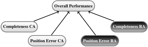
Example 1 Consider the problem of designing an airspace supervision system for Air Traffic Management (ATM). One needs to select the "best" system among several candidate solutions, based on the assessment of their quality [ESASSP, 2012]. In order to make this choice, the decision maker simulates each candidate solution on several scenarios representative of real ATM traffic. The aim of the supervision system is to estimate the trajectories of aircrafts thanks to tracking algorithms. Two elementary attributes are considered to measure the quality of the supervision system: "position error" (Root Mean Square [RMS] error between the estimated trajectories and the real ones), and "completeness" (percentage of the trajectories for which aircrafts are detected and tracked). Attributes position error and completeness are computed separately for the existing classes of aircrafts: CA (Commercial Airplanes) and RA (Recreational airplanes). An MCDA model is then obtained, as shown in Figure 1.
Each scenario depicts a different situation that might occur, and involves a predefined set of trajectories. There are, in particular, scenarios in which there is no aircraft in a given category - e.g. no RA. In this case, this means that there is no evaluation of the two attributes "Position Error RA" and "Completeness RA".
In the previous example, two values of the attributes are missing. In order to assess the candidate solutions on the scenario without RA, one needs a new MCDA model having as attributes only the ones that are evaluated. The corresponding tree appears in Figure 1 in light gray (the nodes in dark gray are removed). It is not realistic to ask the decision maker to calibrate this new model, because of time constraints (the decision maker already spent some significant time to calibrate the full model; one does not wish to spent more time calibrating sub-models), of feasibility (the set of possible missing values might be combinatorial, yielding a combinatorial set of potential sub-models), and of consistency with the original model (there might be unwished important gaps between the original model and the learned restricted one).
1.2 RelatedWorks
In the context of data fusion, missing values can be handled in different ways [Saar-Tsechansky and Provost, 2007; GarcaLaencina et al., 2010]: (1) they can be merely ignored in the fusion process; (2) the missing value can be replaced by a default value, which can be for instance the average value of this variable over a dataset; (3) the fusion mechanism can implicitly take into account missing elements.
In statistics, there are basically three types of missing data: the probability of having a missing value for a variable can be completely random (Missing Completely At Random - MCAR), can be independent of the variable value but dependent on the value of the other variables (Missing At Random - MAR), or can be dependent on the values of all variables (Missing not at Random - NMAR) [Little and Rubin, 2002].
Handling missing data is an important challenge in machine learning [Goodfellow et al., 2016]. The simplest approach consists in completing the missing data by a single value (e.g. the average value over the dataset) [Goodfellow et al., 2016; Lundberg and Lee, 2017]. Other methods fill the gaps with (estimated) probability density functions [Smieja et al., 2018], variational autoencoders [McCoy et al., 2018] or modified generative adversarial network [Yeh et al., 2017].
In Social Choice, when the preferences of the voters are incomplete, a safe approach is to determine whether a candidate is the winner for every possible completion of the preferences - called the necessary winner [Konczak and Lang, 2005]. This idea of robust recommendation is also used in multi-criteria decision making [Boutilier et al., 2004; Wilson, 2014]. If this entailment is empty, one can then compute the proportion of completions which yields each possible outcome [Lahdelma et al., 1998].
The existing works aim at filling the missing values in one way or another. To our knowledge, there is no work in which the missing data is considered as non relevant and shall be removed from the model.
1.3 Contributions
We assume we are given a preference model that has been elicited on the complete set of attributes. Our aim is to automatically construct a sub-model restricted to a subset of attributes, by removing the missing attributes from the original model. Such process is called "restriction operator".
This situation arises in the design of complex system such as in Ex. 1, in which attributes are computed by simulation on operational scenarios. Another application is online monitoring of an industrial system through several Key Performance Indicators (KPIs) measuring the instantaneous performance of the system or its performance over a small interval of time. KPIs are often based on events that occur or not during the time window. A criterion becomes irrelevant if the KPI is a performance attached to events that did not occur.
Section 2 gives the basic definitions. We restrict ourselves to utility models. Three classes of preference models are considered: general quantitative models, monotone quantitative models satisfying normalization conditions, and lastly a versatile class of monotone quantitative models - namely the Choquet integral. This model has many applications in AI, for instance in combinatorial optimization [Galand et al., 2013], incremental elicitation [Benabbou et al., 2017], preference learning [Tehrani et al., 2012], machine leaning with SVM [Li et al., 2015].
The concept of restriction operator is introduced in Section 3. Its expression shall take the form of some kind of combination of the values of the full model for some special alternatives. It is not easy to provide a satisfactory expression of the restriction operator. Hence we start by defining properties that are wished and then we derive the expression of this operator by an axiomatic approach. Axiomatic characterizations are proposed for the three classes of models - see Section 4, 5 and 6 respectively. Different expressions are obtained for these three classes. This first one is linear in the original model and is an average of the model over the missing values. The other two take the form of a normalized average due to the normalization conditions. Moreover the expression of the restriction operator for the last two models differ with regard to the values over which the average is computed.
2 Notation
We consider an MCDA problem with a set N = {1, . . . , n} of attributes. We assume a finite set of values Yi on each attribute i ∈ N. For B ⊆ N, we set YB := ∏i∈B Yi. We assume that the preference model is represented by a quantitative utility over YB. This covers many widely-used models. For model U defined on B, x, y ∈ YB and A ⊆ B, we use the notation U(xA, y-A) to denote the value of U on the compound alternative taking value x on A and value y on B \ A.
The rest of this section is devoted to describing the three classes of models going from the more general one to the less general one.
2.1 General Class of Models
The first class is the family of quantitative preference models. For B ⊆ N, let UG(B) (where G stands for General) be the set of functions U : YB → IR.
We define, for i ∈ N and yi ∈ Yi, the delta function by δyi (xi) = 1 if xi = yi, and δyi (xi) = 0 otherwise.
The Generalized Additive Independence (GAI) model is a very general class of models in class UG(B) that is only supposed to fulfill additivity across subsets of B [Fishburn, 1967; Bacchus and Grove, 1995]. It takes the form
where S is a collection of subsets of B and uS : YS → IR. Note that the additive utility model is a particular case where S contains only singletons [Fishburn, 1970].
Due to the presence of sums in (1), the utility functions shall correspond to scales of difference [Krantz et al., 1971], that is they are given up to an affine transformation. We say that two functions f and g on B are two "equivalent scales" (of difference) - denoted by f ∝B g - if there exists coefficients c1, c0 such that f(xB) = c1 g(xB) + c0.
The following example (taken from [Boutilier et al., 2004]) illustrates the GAI model.
Example 2 The problem is to choose a menu composed of a main dish (attribute 1 with two values {Fish,Meat}) and some wine (attribute 2 with two values {White,Red}). Consider the following GAI model U(x1, x2) = u1(x1) + u1,2(x1, x2) with u1(Fish) = 2, u1(Meat) = 0, u1,2(Fish,White) = 1, u1,2(Fish,Red) = 0, u1,2(Meat,White) = 0, u1,2(Meat,Red) = 1. According to this model, Fish is preferred to Meat, White wine is preferred to Red wine for Fish, and Red wine is preferred to White wine for Meat.
2.2 Monotone Models
In Ex. 2, the preferences over the elements of attribute "wine" are conditional on the value taken on attribute "main dish". Yet we do not encounter such conditional preferences in most of MCDA problems. In this case, there exists a weak order ≿i on each Yi, where xi ≿i yi means that xi ∈ Yi is at least as good as yi ∈ Yi regardless of the values on the other attributes. In Ex. 1, we have such unconditional preferences over the attributes: the smaller the position error the better; the larger the completeness the better. The least preferred and most preferred elements in Yi according to ≿i are denoted by ⊥i and ⊤i respectively. We also set Y i = {⊥i, ⊤i}, and ≻i is the asymmetric part of ≿i. Utility U is said to be "monotone" if U(x) ≥ U(y) whenever xi ≿i yi for all i ∈ N.
The process of removing some criteria A from U makes sense only if the remaining criteria B\A have some influence on U. An attribute i ∈ B is said to be "influential" if there exists xi, yi ∈ Yi and z-i ∈ YB\{i} such that U(xi, z-i) ̸= U(yi, z-i). As U is monotone in its coordinates, we obtain:
We can restrict the previous relation to z-i ∈ Y B\{i}:
In general, (2) does not imply (3). We will only assume (3) in this paper.
We can assume w.l.o.g. that U takes values in [0, 1]. An alternative taking value ⊥i (resp. ⊤i) on all attributes is naturally assigned to the worst (resp. best) possible evaluation 0 (resp. 1). These are two normalization conditions on U.
Definition 1 UM(B) is the set of monotone U ∈ UG(B) fulfilling (3), U(⊥B) = 0 and U(⊤B) = 1.
Example 3 Consider two attributes, Y1 = {a, b, c} (with ⊤1 = c ≻1 b ≻1 a = ⊥1) and Y2 = {a, b, c, d} (with ⊤2 = d ≻2 c ≻2 b ≻2 a = ⊥2) and the normalized monotone utility function U : Y1 × Y2 → IR defined by
| U | a | b | c | d |
| a | 0 | 0 | 0 | 12 |
| b | 0 | 12 | 12 | 12 |
| c | 0 | 12 | 1 | 1 |
2.3 Idempotent Models
We consider the special case, where all attributes are evaluated on the same scale, i.e. Y1 = · · · = Yn =: Y . The values of Y can be interpreted as reference satisfaction levels that have the same interpretation across the criteria. For instance, if value a ∈ Y is interpreted as a bad evaluation, then alternative (a, a, . . . , a) is bad on all criteria and thus deserves the bad evaluation a as overall evaluation. More formally, aggregation function U ∈ UG(B) is said to be "idempotent" if
As U takes values in [0, 1], we shall have Y ⊆ [0, 1]. Not so many aggregation models satisfy this property. The most well-known and versatile class of idempotent aggregation functions is the Choquet integral [Choquet, 1953]. It is a numerical function that applies to numerical values. We restrict ourselves here to the Choquet integral. We assume that Y takes numerical values inside interval [0, 1]: Y = {a0, a1, . . . , ap} with 0 = a0 < a1 < · · · < ap = 1, with ≻i=>. The extreme points of Y are Y = {0, 1}.
The Choquet integral is a versatile model able to represent interaction among criteria [Grabisch et al., 2000; Grabisch and Labreuche, 2010]. It is characterized by a "capacity" [Choquet, 1953] which is a set function µ : 2B → [0, 1] such that µ(∅) = 0, µ(B) = 1 (Normalization conditions) and µ(A) ≤ µ(A′ ) for all A ⊆ A′ ⊆ B (Monotonicity conditions). Criterion i ∈ B is said to be "non-degenerate" in µ if there exists A ⊆ B \ {i} such that µ(A ∪ {i}) > µ(A).
The Choquet integral of x ∈ [0, 1]B w.r.t. a capacity µ has the following expression [Choquet, 1953] :
where τ : {1, . . . , b} → B is a permutation s.t. xτ(1) ≤ · · · ≤ xτ(b), b = |B|, SB τ (j) = {τ(j), . . . , τ(b)}, SB τ (b +1) = ∅.
Definition 2 UC(B) is the set of Choquet integrals on B w.r.t. capacities that are non-degenerate in all criteria.
The Choquet integral satisfies (4). One can readily see that for the Choquet integral, relations (2) and (3) are equivalent and hold iff all criteria are non-degenerate. Hence, due to the monotonicity conditions on capacities, UC(B) ⊆ UM(B).
Model (5) contains many interesting sub-models as particular cases. One of them is the Choquet integral w.r.t. a 2additive capacity. It takes the following expression:
The first part is a weighted sum, where vi represents the mean importance of criterion i. Interaction between criteria comes from the second part. Coefficient Ii,j is the intensity of interaction between criteria i and j, which belongs to [-1, 1]. If Ii,j > 0 (resp. Ii,j < 0), the interaction term penalizes (resp. increases) the overall assessment C 2µ , proportionally to the difference of score between criteria i and j.
Example 4 (Ex. 1 cont.) The elicited model is:
where xji , i ∈ {PE,C} (for Position Error and Completeness resp.) and j ∈ {CA,RA} denote the values of the attributes. Completeness is more important than Position Error as one needs first to track the aircrafts as much as possible, before caring about their position accuracy. Moreover there are positive interactions giving bonus when Completeness and Position Error are simultaneously satisfied, or when the system is good at both CA and RA.
3 Problem Statement
Consider model U ∈ UT(N) where T ∈ {G,M,C}, and alternative x which values are unknown on the attributes A ⊂ N. These values are called "missing". Several approaches can be used to assess the alternative given only x-A. One can model uncertainty on the missing information by the uniform probability distribution over the possible completions of x-A, using the maximum entropy principle. The evaluation of x-A is then obtained by the following expected utility:
We explore here another venue. Given a model elicited on the full set of attributes, we define a restriction operator returning a preference model defined on a subset of attributes. As the process of removing some attributes can be applied several times, the support of the initial model can be a strict subset B of N, and the restricted function shall belong to the same class of models as the initial function. The restriction operator has thus a closed form (with A ⊂ B ⊆ N)
The motivation of using a restriction operator rather than directly a formula such as (7) is twofold. Firstly, it explicitly exhibits a model on the set of attributes with known values. This model can be shown and explained to the user, which is helpful in practice. Secondly, we are interested in the case where all attributes are intrinsically relevant in model U, but an attribute becomes "irrelevant" when its value is unknown (missing). Hence it makes sense to remove the missing attributes and restrict the elicited model.
The rest of this paper is devoted to defining [U]T,B -A (xB\A) for xB\A ∈ YB\A. We adopt an axiomatic approach: instead of starting from an expression (such as (7)), we propose axioms on [·]T,B -A that are important for an end-user, and then we show that there is a unique restriction operator fulfilling these properties. This approach is applied for the three classes of models previously described.
4 Non-Monotone Preference Models
We consider a general model U ∈ UG(B). We first introduce the axioms on [·]G,B -A and then give the axiomatic result.
4.1 Axioms and Axiomatic Result
Linearity
Let us restrict ourselves to the case where A is a singleton A = {i}. The models we consider satisfy some kind of additivity, like for the GAI model (1). If U is a linear combination of two simpler models U ′ and U ′′ , then [U]G,B -i shall be a linear combination of [U ′ ]G,B -i and [U ′′ ]G,B -i . Standard linearity of [·]G,B -i means that [β′ U ′ + β′′ U ′′ ]G,B -i = β′ [U ′ ]G,B -i + β′′ [U ′′ ]G,B -i where β′ , β′′ ∈ IR are constant. Here in order to put β′ , β′′ outside operator [·]G,B -i , it is sufficient that they are constant in i. Hence β′ , β′′ can depend on attributes in B \ {i}.
Axiom Linearity (L): Let B ⊆ N, i ∈ B with B ̸= {i}, β′ , β′′ ∈ UG(B \ {i}), and U ′ , U ′′ ∈ UG(B). Then
Most of MCDA models fulfill some linearity. This ensures a kind of understandability by humans. If the restriction operator were completely non-linear we would obtain a complex and not easy to interpret restricted function.
Proposition 1 Under L, there exists coefficients {γB i (yi)}yi∈Yi such that for all x-i ∈ YB\{i}
Constant
If U is constant, then removing attribute i does not change the function.
Axiom Constant (C): Let B ⊆ N and i ∈ B with B ̸= {i}. If U(x) = C for all x ∈ YB, with C ∈ IR, then [U ]G,B -i (x-i) = C.
Proposition 2 Under L and C, there exists coefficients {γB i (yi)}yi∈Yi such that (9) holds, with
For space limitation, the proofs of this result and others are omitted.
When only one variable needs to be removed, the expression of the restriction operator (see Prop. 2) is similar to a general probabilistic approach computing the expected utility over the unknown values with a non-uniform distribution.
Single Value Contribution
Assume that U ∈ UG(B) takes the form (for i ∈ B and yi ∈ Yi)
Then the result of removing attribute i from U shall not depend on value yi, as stated by the following axiom.
Axiom Single Value Contribution (SVC): Let B ⊆ N, i ∈ B with B ̸= {i}. If U satisfies (11), then [U]G,B -i does not depend on yi.
Proposition 3 Under L, C and SVC, then
The three axioms uniquely specify the restriction w.r.t. one variable, and [U]G,B -i is an average of U over the missing values. We now consider the restriction w.r.t. more variables.
Recursivity
When we need to remove more than one attribute, we can proceed in several ways: remove all of them at the same time, or remove one at a time (with all possible ordering of the variables). There is no reason why these different ways shall provide different outcomes. This idea is expressed in the following axiom defined for T ∈ {G, M, C}.
Axiom Recursivity (R[T]): For all A ⊂ B, i ∈ B \ A with A ∪ {i} ̸= B, and all U ∈ UT(B), we have
Note that this axiom will be used for other assumptions on U, and is thus indexed by T ∈ {G,M, C}.
Theorem 1 [·]G,· -· satisfies L, C, SVC and R[G], if and only if for all B ⊆ N, A ⊂ B and all x-A ∈ YB\A,
This result shows that there is a unique restriction operator fulfilling the four axioms. Interestingly, we recover exactly expression (7) in which the uncertainty on the missing information is modeled by the uniform probability distribution over the possible completions of x-A.
Sketch of the proof: One can easily check that (12) satisfies to all axioms.
Conversely consider [·]G,· -· satisfying all axioms. One can easily show relation (12) by induction on |A|, thanks to Proposition 3 and R[G].
Example 5 (Ex. 2 cont.) We obtain [U]G,N -1 (White) = 12 [U(Fish,White) + U(Meat,White)] = 32 , [U ]G,N -1 (Red) = 1 2 [U(Fish,Red) + U(Meat,Red)] = 32 , [U ]G,N -2 (Fish) = 1 2 [U(Fish, White) + U(Fish, Red)] = 52 , [U ]G,N -2 (Meat) = 1 2 [U(Meat, White) + U(Meat, Red)] = 12 . So there is no intrinsic preference of a particular type of wine, which is consistent with u1,2. Moreover, "fish" is intrinsically preferred to "meat", as expected given u1.
4.2 Justification of the Axioms
In order to see the importance of the axioms, we provide examples of restriction operators violating one axiom and fulfilling the other ones. Note that the existence of such examples also show the independence of the axioms.
This operator satisfies C, SVC and R[G], but violates L. This expression is very simple. It would be a very relevant expression if the aggregation operators were purely ordinal like a weighted min or max operator. However, we are interested in models U having some linearity property. Yet any linearity in U is lost in (13), which can make its expression more complex to understand for the user.
Example 7 Consider
This operator satisfies L, SVC and R[G], but violates C. This relation is not normalized so that [U]G,B -A in (14) is not of the same order of magnitude as for U.
Example 8 Consider
where γB i (yi) = 2 |Yi|+2 if yi ∈ Y i, and γB i (yi) = 1 |Yi|+2 else. This operator satisfies L, C and R[G], but violates SVC. This expression does not treat in a similar way all elements in Yi.
Example 9 Let us define [U ]G,B -A (x-A) = 1 |Yi | ∑yi∈Yi U(yi, x-i) if ∃i ∈ N s.t. A = {i}, and [U ]G,B -A (x-A) = 0 else. This operator satisfies L, C and SVC, but violates R[G]. This expression is not intuitive as what is done for subsets of at least two elements has nothing to do with what is done for singletons.
5 Monotone Preference Models
We now consider monotone models U ∈ UM(B).
Quasi-Linearity
Axiom L cannot be strictly speaking satisfied for functions in UM(B), as [β′ U ′ + β′′ U ′′ ]M,B -i shall be a monotone and normalized aggregation function, which is clearly not the case of β′ [U ′ ]M,B -i +β′′ [U ′′ ]M,B -i when β′ +β′′ ̸= 1 or β′ , β′′ < 0. More precisely, [β′ U ′ + β′′ U ′′ ]M,B -i and β′ [U ′ ]M,B -i + β′′ [U ′′ ]M,B -i shall correspond to two equivalent interval scales. Hence one shall have the next axiom defined for T ∈ {M, C}. Axiom Quasi-Linearity (QL[T]): For B ⊆ N, i ∈ B with B ̸= {i}, U ′ , U ′′ ∈ UT(B), and β′ , β′′ ∈ UG(B \ {i}) with β′ (t), β′′ (t) ≥ 0 ∀t ∈ YB\{i},
Proposition 4 Under QL[T], for B ⊆ N and i ∈ B with B ̸= {i}, there exists coefficients {γB i (yi)}yi∈Yi s.t. [U ]T,B -i (x-i) = GBi (x-i)-GBi (⊥-i) GBi (⊤-i)-GBi (⊥-i) for all x-i ∈ YB\{i}, where GBi (x-i) = ∑yi∈Yi γB i (yi) U(yi, x-i).
Sketch of the proof: The proof uses the fact that if f ∝B g (with f ∈ UT(B), g ∈ UG(B)), then for all xB ∈ YB, f(xB) = g(xB)-g(⊥B) g(⊤B)-g(⊥B) .
Axioms C and SVC do not apply to UM(B). However, assume that U takes the form: U(x) = Ui(xi) × U-i(x-i), with Ui ∈ UM(Yi) and U-i ∈ UM(Y-i). By Proposition 4, GBi (x-i) = [∑yi∈Yi γB i (yi) Ui(yi)] U-i(x-i). If the term in bracket is non null, then [U]M,B -i (x-i) = U-i(x-i)-U-i(⊥-i) U-i(⊤-i)-U-i(⊥-i) = U-i(x-i) as U-i is normalised.
Symmetry
By Prop. 4, the restriction operator on i is a normalized average over terms U(yi, x-i)-U(yi, ⊥-i). The next axiom is a symmetry property saying that [U]T,B -i shall not be modified if we permute these differences over the elements of Yi. We can also multiply these differences by a constant, without any consequence on the restriction.
Axiom Symmetry (S): Let B ⊆ N, i ∈ B with B ̸= {i}, a permutation π on the values of Yi, U,U ′ ∈ UM(B) and C > 0 s.t. for all yi ∈ Yi and x-i ∈ YB\{i}
Without the presence of constant C, there does not exists in general U, U ′ ∈ UM(B) satisfying (15), and thus axiom S would be void.
Adding R[M], we obtain an axiomatization of [·]M,· -· .
Theorem 2 [·]M,· -· satisfies QL[M], S and R[M], if and only if for all B ⊆ N, A ⊂ B and all x-A ∈ YB\A,
For every U ∈ UM(B), this expression is well-defined and belongs to UM(B \ A).
This results shows that there is a unique restriction operator fulfilling the three axioms. The restriction operator is now a normalized sum over all values of the missing attributes.
Sketch of the proof: Under S, the coefficients γB i (yi) are the same for all yi ∈ Yi. To this end, one just needs to show that for all U ∈ UM(B), there exists U ′ ∈ UM(B) satisfying (15).
The end of the proof is similar to that of Theorem 1.
Example 10 (Ex. 3 cont.) The restriction of U to the second attributes is [U]M,{1,2} -1 (t) = F(t) F(c) , where F(t) = (U(a, t) - U(a, a)) + (U(b, t) -U(b, a)) + (U(c, t) -U(c, a)). Then [U ]M,{1,2} -1 (a) = 0, [U]M,{1,2} -1 (b) = 1 2 , [U]M,{1,2} -1 (c) = 34 , [U ]M,{1,2} -1 (d) = 1. On average, the utility of c (resp. b) lies half way in-between b and d (resp. a and d).
6 Monotone Idempotent Preference Model: Case of the Choquet Integral
We now consider elements of UC(B), that is Choquet integrals. These are monotone idempotent aggregation functions.
6.1 Axioms and Characterization Result Quasi-Linearity
We assume property QL[C]. For U ∈ UC(B), [U]C,B -i shall belong to UC(B \ {i}). This implies a stronger result than Proposition 4. More precisely, the sum is only performed on the extreme points 0 and 1, as shown by the following result.
Proposition 5 Under QL[C], there exists coefficients {γN i (yi)}yi∈Y such that
Sketch of the proof: One can show that the expression of Proposition 4 applied on a Choquet integral fulfills idempotency iff γB i (yi) = 0 for yi ∈ Y \ Y .
Symmetry
Symmetry axiom S says that all values of attribute Yi are treated symmetrically. By Proposition 5, only the two extreme values 0 and 1 count. The next axiom restricts S to these extreme values, but is applied only to a subset of cardinality at least 3.
Axiom Symmetry (S'): For B ⊆ N and i ∈ B with |B| ≥ 3, consider U, U ′ ∈ UC(B) s.t. ∀x-i ∈ YB\{i}
Proposition 6 Under QL[C] and S', for all x-i ∈ YB\{i}
Proof : Consider two capacities v and v′ depending only on three attributes i, j, k and xj < xk. Then Cv(1i, x-i) - Cv(1i, 0-i) = xj (v({i, j, k}) - v({i, k})) + xk (v({i, k}) - v({i})) and Cv(0i, x-i) - Cv(0B) = xj (v({j, k}) - v({k})) + xk v({k}). Then if v({i, j, k}) - v({i, k}) = v′ ({j, k})-v′ ({k}) =: dj1 , v({j, k})-v({k}) = v′ ({i, j, k}) - v′ ({i, k}) =: dj0 , v({i, k}) - v({i}) = v′ ({k}) =: dk1 and v({k}) = v′ ({i, k}) - v′ ({i}) := dk0 , then the conditions of S apply for Cv and Cv′ . Then one shall have by Proposition 5
where [Cv]C,B -i (x-i) (resp. [Cv′ ]C,B -i (x-i)) is equal to the left hand side (resp. right hand side) of this relation. As this shall hold for every dj1 , dj0 , dk1 , dk0 (small enough), and xj < xk, we conclude that γN i (1) = γN i (0).
Theorem 3 [·]C,· · defined for B ⊆ N, A ⊂ B and U ∈ UC(B) satisfies QL[C], R[C] and S' if and only if for all B ⊆ N, A ⊂ B with A ̸= B, and all U ∈ UC(B)
where F B A (x-A) = ∑D⊆A U(1D, 0A\D, x-A). Moreover for every function in UC(B), (16) is well-defined and belongs to UC(B \ A).
This results shows that there is a unique restriction operator fulfilling the three axioms. The restriction operator is a normalized sum over the extreme points 0 and 1 of the missing attributes.
Proof : One can easily verify that (16) satisfies QL[C], R[C] and S'. The "only if" part of the theorem is provided by combining Proposition 6, and proceeding as in Theorem 1.
Consider U ∈ UC(B), A ⊂ B and k ∈ B\A. By (3), there exists D ⊆ B\(A∪{k}) such that U(1D, 0B\(D∪{k}), 1k) > U(1D, 0B\(D∪{k}), 0k). By monotonicity of U, this yields
Hence the denominator of (16) is always non-zero, so that (16) is well-defined for every function in UC(B).
6.2 Interpretation
The next result provides the expression of the restriction operator for a two-additive Choquet integral.
Theorem 4 For a two additive Choquet integral U defined on B with importance and interaction indices vi and Ii,j respectively, [U]C,B -A is also a two-additive Choquet integral with the following importance and interaction terms:
Expressions (17) are very intuitive and simpler to compute than (16). The relative importance between criteria in B \ A remain the same. Hence, in order to get an idempotent model, the weight vi is divided by ∑k∈B\A vk. The interaction index between two criteria in B \ A is simply the previous interaction divided by the same factor. The other interactions are merely discarded, as expected.
Example 11 (Ex. 4 cont.) Attributes xRA PA and xRA C are unknown (see Ex. 1). By Theorem 4, the restriction [U]-RA of U (defined in Ex. 4) to the remaining two attributes is
Comparing to the expression of U, we keep only the terms for which the variables are known (namely xCA C and xCA PE ). As for U, C is twice as more important than PE, and there is a strong positive interaction between C and PE. Expression [U]-RA thus completely makes sense.
7 Discussion and Perspectives
This paper addresses the problem of how to handle missing data interpreted as non-relevant, in a preference model. More specifically, given a model defined on the full set of attributes, we have defined a restriction operator returning a preference model defined on a subset of attributes. Axiomatic characterizations are proposed for three classes of models. For general quantitative models, the restriction operator is characterized by linearity, recursivity and particular cases of constant models and models depending only on one variable. We obtain the average of the value of the utility over all possible values of the missing attributes. The second class is the set of monotone quantitative models satisfying normalization conditions. The linearity axiom is changed to fit with these conditions. Adding recursivity and symmetry, we obtain a normalized average of the utility over all values of the missing criteria. The last class is the Choquet integral w.r.t. non-degenerate capacities. With the same axiom as before, we obtain a simpler expression averaging only on the extreme values of the missing criteria. Finally, a very intuitive interpretation is provided for two-additive Choquet integrals.
Our approach has advantages over the existing ones. A robust approach is too pessimistic. In Ex. 1, it would penalize a system when the values of the two attributes are missing. There is no reason to do so as there is no RA in the scenario. The drawback of the probabilistic approach is on the assumptions made for the completion of the missing data. However, it is interesting to note that it yields exactly the same expression as in our approach for the non-monotone model (see Theorem 1). The main asset of our approach is that it brings a strong axiomatic justification.
If a naive approach works well for the non-monotone case, it is not the case for the other models. We have shown that for monotone models, one shall use a normalized average rather than a simple average to get a consistent result, and that for the Choquet integral, we shall only consider the extreme points. These major points are derived by the axiomatic approach and the closed form of the restriction operator.
The paper can be extended in several directions. Theorems 2 and 3 are not strictly speaking expected utility. It would be interesting to investigate whether it can be put under the form of a conditional expectation, with the denominator being the expected utility of the conditioned event. The idea of removing missing data can be adapted to other fields such as machine learning or data fusion. Applying a learned (classification/regression) model when attributes are missing while still requiring a precise prediction requires to make strong assumption about the missingness process, such as MAR, NMAR. Our current approach provides an alternative way to handle missing attributes by simply removing it from the model, allowing one to make predictions without assumptions about the missingness process.
Acknowledgments
This work has been supported by the European project SESAR H2020 PJ14.04.03 EECNS: "Essential and Efficient Communication Navigation and Surveillance Integrated System".
@inproceedings{ijcai2019p243,
  title     = {How to Handle Missing Values in Multi-Criteria Decision Aiding?},
  author    = {Labreuche, Christophe and Destercke, Sébastien},
  booktitle = {Proceedings of the Twenty-Eighth International Joint Conference on
               Artificial Intelligence, {IJCAI-19}},
  publisher = {International Joint Conferences on Artificial Intelligence Organization},
  editor    = {Sarit Kraus},
  pages     = {1756--1763},
  year      = {2019},
  month     = {8},
  note      = {Main track},
  doi       = {10.24963/ijcai.2019/243},
  url       = {https://doi.org/10.24963/ijcai.2019/243},
}
TY - CPAPER TI - How to Handle Missing Values in Multi-Criteria Decision Aiding? AU - Labreuche, Christophe AU - Destercke, Sébastien T2 - Proceedings of the Twenty-Eighth International Joint Conference on Artificial Intelligence, IJCAI-19 PB - International Joint Conferences on Artificial Intelligence Organization PY - 2019 SP - 1756 EP - 1763 DO - 10.24963/ijcai.2019/243 UR - https://doi.org/10.24963/ijcai.2019/243 ER -Copied
Machine-readable versions of this paper, for tools and AI agents:





