
Recommending Links to Maximize the Influence in Social Networks
Proceedings of the Twenty-Eighth International Joint Conference on Artificial Intelligence. Main track. Pages 2195-2201.
https://doi.org/10.24963/ijcai.2019/304
Keywords
- Machine Learning Applications: Networks
- Multidisciplinary Topics and Applications: Social Sciences
- Machine Learning: Recommender Systems
- Machine Learning: Data Mining
Abstract
Social link recommendation systems, like "People-you-may-know" on Facebook, "Who-to-follow" on Twitter, and "Suggested-Accounts" on Instagram assist the users of a social network in establishing new connections with other users. While these systems are becoming more and more important in the growth of social media, they tend to increase the popularity of users that are already popular. Indeed, since link recommenders aim at predicting users' behavior, they accelerate the creation of links that are likely to be created in the future, and, as a consequence, they reinforce social biases by suggesting few (popular) users, while giving few chances to the majority of users to build new connections and increase their popularity.In this paper we measure the popularity of a user by means of its social influence, which is its capability to influence other users' opinions, and we propose a link recommendation algorithm that evaluates the links to suggest according to their increment in social influence instead of their likelihood of being created. In detail, we give a constant factor approximation algorithm for the problem of maximizing the social influence of a given set of target users by suggesting a fixed number of new connections. We experimentally show that, with few new links and small computational time, our algorithm is able to increase by far the social influence of the target users. We compare our algorithm with several baselines and show that it is the most effective one in terms of increased influence.
- [Adamic and Adar, 2003] Lada A. Adamic and Eytan Adar. Friends and neighbors on the web. Social Networks, 25(3):211-230, 2003.
- [Arnetminer, 2015] Arnetminer. Arnetminer. http://arnetminer.org, 2015. Accessed: 2015-01-15. Link
- [Boldi and Vigna, 2014] Paolo Boldi and Sebastiano Vigna. Axioms for centrality. Internet Mathematics, 2014.
- [Bollobás et al., 2003] Béla Bollobás, Christian Borgs, Jen- nifer T. Chayes, and Oliver Riordan. Directed scale-free graphs. In 14th SODA, pages 132-139, 2003.
- [Chaoji et al., 2012] Vineet Chaoji, Sayan Ranu, Rajeev Rastogi, and Rushi Bhatt. Recommendations to boost con- tent spread in social networks. In 21st World Wide Web Conference 2012, WWW, pages 529-538, 2012.
- [Chen et al., 2010] Wei Chen, Yifei Yuan, and Li Zhang. Scalable influence maximization in social networks under the linear threshold model. In 10th International Confer- ence on Data Mining, pages 88-97, 2010.
- [Cohen et al., 2014] Edith Cohen, Daniel Delling, Thomas Pajor, and Renato F. Werneck. Sketch-based influence maximization and computation: Scaling up with guaran- tees. In 23th CIKM, pages 629-638, 2014.
- [Crescenzi et al., 2016] Pierluigi Crescenzi, Gianlorenzo D'Angelo, Lorenzo Severini, and Yllka Velaj. Greed- ily improving our own closeness centrality in a network. TKDD, 11(1):9:1-9:32, 2016.
- [D'Angelo et al., 2016] Gianlorenzo D'Angelo, Lorenzo Severini, and Yllka Velaj. Influence maximization in the independent cascade model. In 17th Italian Conference on Theoretical Computer Science., pages 269-274, 2016.
- [D'Angelo et al., 2019] Gianlorenzo D'Angelo, Lorenzo Severini, and Yllka Velaj. Recommending links through influence maximization. Theor. Comput. Sci., 2019.
- [Eirinaki et al., 2018] Magdalini Eirinaki, Jerry Gao, Iraklis Varlamis, and Konstantinos Tserpes. Recommender sys- tems for large-scale social networks: A review of chal- lenges and solutions. Future Generation Comp. Syst., 78:413-418, 2018.
- [Jaccard, 1901] Paul Jaccard. Étude comparative de la distri- bution florale dans une portion des alpes et des jura. Bull Soc Vaudoise Sci Nat, 37, 1901.
- [Kempe et al., 2015] David Kempe, Jon M. Kleinberg, and Éva Tardos. Maximizing the spread of influence through a social network. Theory of Computing, 11:105-147, 2015.
- [Khalil et al., 2014] Elias Boutros Khalil, Bistra N. Dilkina, and Le Song. Scalable diffusion-aware optimization of network topology. In 20th KDD, pages 1226-1235, 2014.
- [Kimura et al., 2008] Masahiro Kimura, Kazumi Saito, and Hiroshi Motoda. Solving the contamination minimization problem on networks for the linear threshold model. In 10th PRICAI, pages 977-984, 2008.
- [Kuhlman et al., 2013] Chris J. Kuhlman, Gaurav Tuli, Samarth Swarup, Madhav V. Marathe, and S. S. Ravi. Blocking simple and complex contagion by edge removal. In 13th ICDM, pages 399-408, 2013.
- [Kunegis, 2013] Jérôme Kunegis. Konect: the koblenz net- work collection. In 22nd International Conference on World Wide Web, pages 1343-1350, 2013.
- [Li et al., 2018] Zhepeng (Lionel)
- Li, Xiao Fang, and Olivia R. Liu Sheng. A survey of link recommendation for so- cial networks: Methods, theoretical foundations, and fu- ture research directions. ACM Trans. Management Inf. Syst., 9(1):1:1-1:26, 2018.
- [Liben-Nowell and Kleinberg, 2007] David Liben-Nowell and Jon M. Kleinberg. The link-prediction problem for social networks. JASIST, 58(7):1019-1031, 2007.
- [Nemhauser et al., 1978] George L. Nemhauser, Lau- rence A. Wolsey, and Marshall L. Fisher. An analysis of approximations for maximizing submodular set functions -I. Math. Program., 14(1):265-294, 1978.
- [Newman, 2001] Mark EJ Newman. Clustering and prefer- ential attachment in growing networks. Physical review E, 64(2):025102, 2001.
- [Papagelis, 2015] Manos Papagelis. Refining social graph connectivity via shortcut edge addition. TKDD, 10(2):12:1-12:35, 2015.
- [Parotsidis et al., 2016] Nikos Parotsidis, Evaggelia Pitoura, and Panayiotis Tsaparas. Centrality-aware link recommen- dations. In 9th WSDM, pages 503-512, 2016.
- [Sanz-Cruzado and Castells, 2018] Javier Sanz-Cruzado and Pablo Castells. Enhancing structural diversity in social networks by recommending weak ties. In 12th Conference on Recommender Systems, RecSys, pages 233-241, 2018.
- [Sheldon et al., 2012] Daniel Sheldon, Bistra N. Dilkina, Adam N. Elmachtoub, Ryan Finseth, Ashish Sabharwal, Jon Conrad, Carla P. Gomes, David B. Shmoys, William Allen, Ole Amundsen, and William Vaughan. Maximiz- ing the spread of cascades using network design. CoRR, abs/1203.3514, 2012.
- [Stoica et al., 2018] Ana-Andreea Stoica, Christopher J. Riederer, and Augustin Chaintreau. Algorithmic glass ceiling in social networks: The effects of social recom- mendations on network diversity. In 27th WWW, pages 923-932, 2018.
- [Su et al., 2016] Jessica Su, Aneesh Sharma, and Sharad Goel. The effect of recommendations on network struc- ture. In 25th International Conference on World Wide Web, WWW, pages 1157-1167, 2016.
- [Wu et al., 2015] Xiaojian Wu, Daniel Sheldon, and Shlomo Zilberstein. Efficient algorithms to optimize diffusion pro- cesses under the independent cascade model. NIPS Work. on Networks in the Social and Information Sciences, 2015.
- [Zhang et al., 2015] Yao Zhang, Abhijin Adiga, Anil Vul- likanti, and B. Aditya Prakash. Controlling propagation at group scale on networks. In International Conference on Data Mining, ICDM, pages 619-628, 2015.
References were extracted automatically from the PDF and may contain errors.
Full text extracted automatically from the PDF; figures, tables and equations may differ. The PDF is the version of record.
1 Introduction
Nowadays, recommendation system has become a key ingredient to boost social networks revenue. These systems help users decide which product to buy, news to read, or which movie to watch. Their combination with online social networks opens up new opportunities for product marketing as well as improving the user experience helping them to make new friends and therefore be exposed to more information. Indeed, adding new connections between users increase the capabilities of a social network of spreading information which in turn increases the retention rate and the number of new subscriptions. In fact, the capability of a user to spread information, usually called social influence, is directly correlated with both the user engagement and its revenue [Chaoji et al., 2012]. Being able to quickly and effectively reach a large number of people by sharing content helps a user to express and diffuse its own opinion, and to discover novel contents and information. At the same time, this increases the chances of making profits from advertisement.
∗Contact Author
Most of the existing link recommendation systems do not consider the impact of the new links on social influence, which is crucial for both users and social networks. Instead, they exploit similarity metrics of user profiles and structural network properties to estimate the likelihood that a link is adopted by users. Based on this estimation, they recommend links that are likely to be established; we point the reader to a recent survey [Li et al., 2018]. For example, the Friend-ofFriend algorithm [Liben-Nowell and Kleinberg, 2007] suggests links towards the users that have the highest number of common friends with the receiver of the recommendation. While these approaches are accelerating the growth of social networks, they are also altering their structure, amplifying the popularity of well-known users and reinforcing social biases and under-representation of demographic groups, respect to their natural growth [Sanz-Cruzado and Castells, 2018; Stoica et al., 2018; Su et al., 2016].
In this paper we look at social influence as a measure of users' popularity and propose a link recommendation algorithm that focuses on links that increase the social influence of a target group of users. We formulate the link recommendation task as an optimization problem that asks to suggest a fixed number of new connections to a subset of users with the aim of maximizing the network portion that is reached by their generated content.
1.1 RelatedWork
There exist an extensive literature on the problem of recommending links to users of a social networks [Li et al., 2018; Eirinaki et al., 2018]. However, there are only few studies on the problem of adding links in a network considering social influence. In the following, we focus on two widely studied diffusion models, the Independent Cascade Model (ICM) and the Linear Threshold Model (LTM) [Kempe et al., 2015], and review papers that study network modification problems in these models. ICM has been considered in several studies. D'Angelo et al. [2019] introduced the Influence Maximization with Augmentation problem (IMA) that consists in adding a limited number of edges incident to a given set of nodes in order to maximize their capability of spreading information. They proved that such problem is NP-hard to approximate within a factor greater than 1-1/2e and provide an approximation algorithm that almost matches such upper bound. Sheldon et al. [2012] study the problem of adding nodes in a network to maximize the diffusion in a network. They show that their problem is not submodular and propose exact integer programming formulations. Wu et al. [2015] considered other types of graph modifications such as modifying the probability of infect other nodes, however, they show that the problem is NP-hard and is neither sub- nor super-modular.
We now review papers on network modification problems under LTM. Heuristics for the edge removal problem have been studied in [Kuhlman et al., 2013; Kimura et al., 2008] but without providing an approximation guarantee. Khalil et al. [Khalil et al., 2014] consider two types of graph modification, adding/deleting edges in order to minimize the information diffusion showing that this network structure modification problem has a supermodular objective and therefore can be solved by algorithms with proven approximation guarantees. Zhang et al. [2015] consider the problem removing edges and nodes with the aim of minimizing the information diffusion and develop algorithms with rigorous performance guarantees and good empirical performance. Experimental studies show that increasing the connectivity or the centrality of a node, by adding edges to the graph, lead also to an increase in the expected number of nodes that the diffusion process is able to reach [Crescenzi et al., 2016; Parotsidis et al., 2016; Papagelis, 2015].
Our Contribution We consider the IMA problem introduced in [D'Angelo et al., 2019]. We first focus on the LTM model of diffusion and show that the objective function is monotone and submodular. We exploit this property to show that a greedy algorithm guarantees a 1 - 1/e approximation. We then propose several techniques that heuristically speed up the running time of our algorithm and of that in [D'Angelo et al., 2019]. We test our algorithms in several random and real-world networks, showing that they are able to substantially increase the spreading capabilities of the target nodes and outperform many alternative baselines.
2 Notation and Problem Statement
In this section, we first define the information diffusion models used in the paper, and then introduce the IMA problem and the related notation.
2.1 Information DiffusionModels
A social network is represented by a weighted directed graph G = (V, E, w), where nodes V represent users, edges E represent relationships between users, and the weight function w : V × V → [0, 1] represents the influence between users. Let Nv denote the set of the in-neighbors of node v ∈ V .
Both ICM and LTM models distinguish between nodes that spreads information, called active, and all the others, called inactive. Active nodes are the ones that, with some probability, diffuse the information to their neighbors. The ICM model requires a diffusion probability to be associated with each edge, whereas LTM requires an influence degree to be defined on each edge and an influence threshold on each node. For both models, the diffusion process proceeds iteratively in a synchronous way along a discrete time-axis, starting from an initial set of nodes, usually called seeds. The process terminates when no further node gets activated.
Kempe et al. showed that the distribution of the set of active nodes in the graph starting from the seed set nodes, usually denoted as A0, under both the ICM and LTM process is equivalent to the distribution reachable from the same set A0 in the set of random graphs called live-edge graphs (Theorem 4.5, 4.6 in [Kempe et al., 2015]), since the processes are point-wise identical, also the expected number of activated nodes is the same. Given a graph G = (V,E,w), a live-edge graph G′ = (V,E′ ), where E′ ⊆ E, is built as follows: (ICM) Every edge (u, v) ∈ E is selected to be inserted to E′ independently at random with a probability proportional to its weight wuv; (LTM) every node v ∈ V , independently, picks at most one of its incoming edges with probability equal to the weight of that edge: edge (u, v) ∈ E is selected with probability wuv, and no edge is selected with probability 1 - ∑(u,v)∈E wuv .
Moreover, evaluating the expected number of active nodes is #P-complete [Chen et al., 2010], however it can be efficiently approximated by using a polynomial number liveedge graph: Kempe et al. proved that, by applying a multiplicative form of the Chernoff bound, we can get (1 ± ǫ)- approximation to the expected number of active nodes, with high probability ([Kempe et al., 2015, Proposition 4.1]).
2.2 Problem Statement
Given a directed graph G = (V,E,w), a budget B ∈ N and a set A ⊆ V of seed nodes consider a larger graph ¯G = (V, ¯E,w) where ¯E contains all the edges in E and, in addition, it contains all the remaining pairs between nodes in A and any other node in V , namely, ¯E = E ∪ (A × V ) with the constraint that ∑(u,v)∈ ¯E wuv ≤ 1 for any node v ∈ V .
For a set S of edges in ¯E\E, let us denote by G(S) the graph augmented with the set of edges S, i.e. G(S) = (V,E ∪ S). In the Influence Maximization with Augmentation problem (IMA) we aim at finding a set S ⊆ ¯E\E of size B in order to maximize the expected number of active nodes in G(S) at the end of the ICM or LTM process. Let us denote by G(S) the set of all possible live-edges sampled fromG(S), then we denote as σ(A, S) := ∑G′∈G(S) P(G′ ) |RA(G′ )| the expected number of activated nodes at the end of the process with seed nodes A in graph G(S), where, RA(G′ ) is the set of reachable nodes from nodes in A in graph G′ , i.e., RA(G′ ) = {u ∈ V : ∃ path from v ∈ A to u ∈ G′ }. Thus, the IMA problem consists in finding a set S∗ such that
The IMA Problem Under ICM Here we review previous results on the IMA problem under ICM. The problem was originally introduced in [D'Angelo et al., 2016], where the authors defined a preliminary version of the IMA problem in which the set of seed nodes is a singleton and presented a constant factor approximation algorithm for that case. In [D'Angelo et al., 2019] they extended the original problem without restrictions on the seed set size. Namely, they studied the problem of adding a set of edges incident to an arbitrary set of initial seeds, without exceeding a given budget, in order to maximize the number of nodes that eventually become active. Moreover, they consider the case in which the cost of any single edge is a value between [0, 1]. They first proved that under ICM and with unitary cost on the edges the IMA problem is NP-hard to be approximated within a constant factor greater than 1 - (2e)-1 . For this case, they provide a greedy based algorithm that guarantees a 1 - e-1 - ǫ approximation factor. This result has been obtained by proving that the objective function σ(A, S) is monotone and submodular w.r.t. set S, and hence the greedy algorithm in [Nemhauser et al., 1978] can be used to obtain the mentioned approximation ratio. They extend this result to the general cost case by using an enumeration technique.
3 Approximation for IMA under LTM
In this section, we first prove that the function σ(A, S) under LTM is monotone and submodular w.r.t. to the set of added edges S and then we exploit this property to provide a constant approximation algorithm for the IMA problem.
Le us denote by G the set of all possible live-edge graphs sampled from graph G. For every live-edge graph G′ = (V,E′ ) ∈ G we denote by P(G′ ) the probability that G′ is sampled, and by p(v, G′ ) the probability for a node v ∈ V of having an incoming edge in G′ . Therefore, p(v,G′ ) is either equal to wuv if there exists an edge (u, v) ∈ E′ , for some u ∈ Nv, or p(v,G′ ) = 1 - ∑(u,v)∈E wuv if no edge is selected. Then we can easily extend this notation to a set of nodes V ′ ⊆ V as p(V ′ ,G′ ) = ∏v∈V ′ p(v,G′ ). Thus,
Finally we denote as PS (G′ ) = p(V, G′ , S) the probability of a live-edge graph G′ ∈ G(S), where G(S) is the set of all possible live-edge graphs sampled from graph G(S).
We first fix the following observation: Consider the probability of a live-edge G′ sampled from G(S ∪ {e}) and a second live-edge graph G′′ ∈ G(S) when adding a new edge e = (a, v) in G(S). Probabilities PS∪e (G′ ) and PS (G′′ ) differ only in the calculation concerning node v, since all the other nodes have the same set of possible in-neighbors with the same set of weights. Therefore, we have 3 cases:
- For any live-edge graph G′ ∈ G(S ∪ e) that selects an edge different from e as incoming edge to v there exists a corresponding G′′ ∈ G(S) with the same edge set, therefore we have that PS∪e (G′ ) = PS (G′′ );
- For any live-edge graph G′ ∈ G(S ∪ e) in which no incoming edge is selected for the node v
- there exists a corresponding G′′ ∈ G(S) with the same edge set. In this case PS∪e (G′ ) = p(V \{v},G′ , S)(1 - ∑z∈Nv wzv - we) and PS (G′′ ) = p(V \{v},G′′ , S)(1 - ∑z∈Nv wzv), where p(V \{v}, G′ , S) = p(V \{v}, G′′ , S);
- For any live-edge graph G′ ∈ G(S ∪ e), G′ = (V,E′ ), that selects e as incoming edge to v we have that PS∪e (G′ ) = p(V \{v},G′ , S)we. Note that, in this case we have |RA(G′ )| ≥ |RA(G′′ )|, for any live-edge graph G′′ ∈ G(S) with edge set E′\{e}.
We can now prove the following theorem.
Theorem 1. Given a graph G = (V, E), σ(A, (V, E ∪ S)) is a monotone submodular function of S ⊆ ¯E\E.
Proof. We first prove that σ(A, ·) is a monotonically increasing function, formally σ(A, S ∪ {e}) ≥ σ(A, S) for any S ⊆ ¯E\E and e = (u, v) ∈ ¯E\E.
We decompose σ(A, S ∪ {e}) as the sum over all the liveedge graphs in which: an edge in E has been selected; v has no incoming edges; and edge e has been selected. Formally, 1
Similarly we have that σ(A, S) can be decomposed as: σ(A, S) = ∑ G′′∈G(S) s.t.∃(z,v)∈E′′ PS (G′′ ) |RA(G′′ )| + ∑ G′′∈G(S) s.t.̸∃(z,v)∈E′′ PS (G′′ ) |RA(G′′ )|.
Using observation 1 and 2 we can consider pair of liveedge graphs, one from G(S ∪ e) and one from G(S), and notice that the two graphs are equivalent in the case in which an edge different from e is selected or node v has no incoming edges. Although, in the latter case the probabilities to sample the live-edge graph aare not equal. Thus, we have that
Thus, we have that σ(A, S ∪ {e}) - σ(A, S) = ∑ G′∈G(S) s.t.̸∃(z,v)∈E′ p(V \{v}, G′ , S)we(|RA(G′′′ )| - |RA(G′ )|),
where G′′′ is the graph G′ augmented with the edge e and the number of live-edge graphs such that the edge e has been selected is the same as the number of live-edge graphs for which no incoming edge is selected for v. Note that this value is greater or equal than zero because |RA(G′′ )| ≥ |RA(G′ )|.
1E′ and E′′ denote the edges sets of graphs G′ and G′′ , resp.
In order to prove that the function is submodular, we show that for each pair of sets S, T such that S ⊆ T ⊂ ¯E\E and for each e = (a, v) ∈ ¯E\(T ∪ E), σ(A, S ∪ {e}) - σ(A, S) ≥ σ(A, T ∪ {e}) - σ(A, T). Let V ′ be the set of nodes that have an incoming edge from the set T\S, namely, V ′ = {v : (w, v) ∈ T\S}. Observe that for any live-edge graph G′ ∈ G(S) for which the nodes in V ′ have no incoming edges there exists G′1 , . . . ,G′ℓ ∈ G(T) such that G′ ⊆ G′i for any i = 1, . . . , ℓ and RA(G′ ) ⊆ RA(G′i ), where ℓ = 2|T\S| . While for all graphs G′ ∈ G(S) that have at least an edge incoming a node in V ′ , there exists a corresponding live-edge graph G′′ ∈ G(T) that is sampled with the same probability as G′ . In the former case, instead, we have that the probability for each G′i , i = 1, . . . , ℓ, is equal to the probability of the corresponding live-edge G′ in G(S) in which no incoming edge is selected for the nodes in V ′ . Formally we have that PS (G′ ) = p(V \V ′ , G′ , S) ∏v∈V ′ (1-∑z∈Nv wzv) and PT (G′i ) = p(V \V ′ , G′ , S) · p(V ′ , G′ , T\S), where
Finally we can write the difference in the increment when adding the edge e = (a, v) in the set T as follow:
that is equal to σ(A, S ∪ {e}) - σ(A, S), where G′′ is the graph G′ augmented with the edge e.
Thus, we can use a simple greedy algorithm (reported in Algorithm 1) to find a set S of edges whose value σ(A, S) is at least 1 - 1/e times the one of an optimal solution for the IMA Problem. The algorithm iterates B times and, at each iteration, it adds to an initially empty solution S an edge ˆ e = (ˆa, ˆ v) s.t. (ˆa, ˆ v) ∈ ¯E\E that gives the maximum marginal increment of the value of σ(A, S). Note that we are not able to compute exactly the value of σ(A, S) in polynomial time but, with probability 1 - δ, we can compute an
Algorithm 1 Greedy algorithm for IMA.
Require: Graph G = (V, E, w); Seed set A; Budget B
- 1: for i = 1, 2, . . . ,B do
- 2: for each e ∈ ¯E\(E ∪ S) do
- 3: Use repeated sampling to estimate a (1 + λ)- approx. of σ(A, S ∪ {e}) with prob. 1 - δ
- 4: Let ˜σ(A, S ∪ {e}) be the estimation
- 5: ˆ e=argmax{˜σ(A, S∪{e})|e=(a, v) ∈ ¯E\(E∪S)}
- 6: S := S ∪ {ˆ e}
- 7: return S
1 + λ approximation of it by sampling a polynomial number of live-edge graphs, for any λ and δ [Kempe et al., 2015]. We then exploit the result of Nemhauser et al. that allows us to analyze the greedy algorithm in the case of monotone submodular objective functions that can be approximately evaluated [Nemhauser et al., 1978]. The next corollary follows.
Corollary 1. Algorithm 1 guarantees an approximation factor of (1- 1e -ǫ) for the IMA problem, where ǫ is any positive real number.
The computational complexity of Algorithm 1 is O(B · |V | · g(|V |, |E| + B)), where g(|V |, |E| + B) is the complexity of computing an approximation ˜σ(A, S) of σ(A, S) in a graph with |V | nodes and |E| + B edges. More precisely, it runs in B iterations, each of which requires estimating the expected spread of O(|V |) node sets. Since g(|V |, |E| + B) = O(|E| · R) where R is the number of simulations, then the complexity of the greedy algorithm is O(B · |V | · |E| · R) which is clearly infeasible, in terms of running time, for very large real networks.
4 Improving the Running Time
In what follows we propose some techniques to heuristically reduce the running time of the greedy algorithm. Note that this techniques can be applied to the greedy algorithm proposed in [D'Angelo et al., 2019] and to Algorithm 1. In Section 5 we evaluate an implementation of the algorithm that exploits a combination of these heuristics.
- Exploiting submodularity. Since σ(A, S) is submodular, we have that the increment to the expected number of active nodes after adding an edge e to G(S) is monotonic non-increasing. Thus, the increment is upper bounded by any solution S′ ⊆ S with the addition of the new edge e, that is σ(A, S′ ∪ {e}) - σ(A, S′ ) ≥ σ(A, S ∪ {e}) - σ(A, S). We can exploit this property in Algorithm 1 to reduce the computational complexity of our algorithm. Consider the loop at line 1 for any iteration i ≥ 2 and for some edge e, we check if the increment found so far is greater than the increment in the previous iteration, i.e., i - 1, with the edge e. In this case, in fact, we know that the edge e cannot increase the value of σ(A, S) more than the maximum found so far. Therefore, in this case we prune the search.
- Live-edge graph reduction. At the end of each iteration of the loop at line 1 of Algorithm 1, we reduce the size
of all the live-edge graphs by removing the nodes that become influenced when adding an edge to the solution. Reducing the size after each iteration reduces the time required to compute ˜σ(A, S ∪ {e}) for each new edge e.
- Low probability candidate edge pruning. The greedy algorithm needs to compute ˜σ(A, S ∪ {e}) for each e ∈ ¯E\(E ∪ S) to find an edge that maximizes this quantity. However, if we have that wa1u > wa2u for some nodes a1, a2 ∈ A and u ∈ V \A, then σ(A, S ∪ {a1, u}) > σ(A, S ∪ {a2, u}). Thus, in the loop of line 2 we only consider, for each u ∈ V \A, the edge (a, u) ∈ ¯E\(E ∪ S) with the highest weight.
- Reduction to Limited Seed Selection. Given a weighted directed graph with edge weights capturing influence probabilities (in ICM or LTM), an integer B′ , and two sets of nodes A,L ⊆ V , the Limited Seed Selection problem (LSS) aims to to find a set of B′ users S ⊆ L such that, by targeting S ∪ A, the expected number of influenced users is maximum. Nodes in S are excluded from the objective function.
Problems IMA and LSS have the same objective function, but the former looks for a set of edges, while the later looks for a set of nodes to be added to a give set of seeds. In what follows we describe how to transform an instance IIMA of the IMA problem into an instance ILLS of the LSS problem and how to transform a solution SLSS for ILLS into a solution SIMA for IIMA with the same value. Given IIMA = (G,A,B), we define ILSS = ( ˆG,L,B) where ˆG = (ˆ V , ˆE, ˆw) is a graph obtained by adding |L| = |V \A| · |A| nodes and edges to G. Formally, let L = ∪a∈ALa be the additional nodes, where |Li| = |V \A| and La ∩ Lb = ∅, for each a, b ∈ A, a ̸= b. Then, ˆ V = V ∪ L and ˆE = E ∪ ⋃a∈A(La × (V \A)). The weights of the new edges are equal to that of the corresponding edges in ¯E\E, i.e. ˆwa′ v = wav, for each a ∈ A, a′ ∈ La, and v ∈ V \A. Any solution SLSS for ILSS is made of nodes in L and each of these nodes corresponds to unique edge in G, we define SIMA accordingly. We denote with σG and σ ˆG the expected number of influenced nodes in G and ˆG, respectively. The next theorem show that the two solutions have the same value. 2
Theorem2. In both ICMand LTM, σ ˆG(A∪SLSS, ∅) = σG(A, SIMA) + B.
Thanks to Theorem 2, we can use any algorithm for LSS to solve IMA. Problem LSS is different from the influence mazimization problem in [Kempe et al., 2015]. However, many algorithm for this latter can be easily adapted for solving LSS. In particular, we adapt the algorithm presented in [Cohen et al., 2014] such that it finds a seed set S⊆L, given a limited set of nodes L.
5 Experimental Study
In this section we experimentally evaluate the performance of our greedy algorithm and of that in [D'Angelo et al., 2019].
2 Note that the objective function of LSS is σ ˆG(A∪SLSS, ∅)-B.
| Name | |V | | |E| |
|---|---|---|
| Software Engineering (SE) | 3,141 | 14,787 |
| Theoretical CS (TCS) | 4,172 | 14,272 |
| High-Performance Comp. (HPC) | 4,869 | 35,036 |
| Wiki-Vote (Wiki) | 7,115 | 103,689 |
| Computer Graphic (CGM) | 8,336 | 41,925 |
| Computer Networks (CN) | 9,420 | 53,003 |
| Artificial Intelligence (AI) | 27,617 | 268,460 |
| Slashdot (Sl) | 51,083 | 130,370 |
| Epinions (Epi) | 75,879 | 508,837 |
| Slashdot-Zoo (Sl-z) | 79,116 | 515,397 |
| Digg | 279,630 | 1,731,653 |
| Citeseer | 384,413 | 1,751,463 |
| 465,017 | 834,797 |
For both ICM and LTM, we implemented two versions of these algorithms: GREEDY1 exploits the first three heuristics described in the previous section; and GREEDY2 exploits the reduction to LSS. We compare the number of activated nodes in a graph augmented by using the greedy solution with the number of activated nodes in the original graph and in the graph augmented by using several alternative baselines.
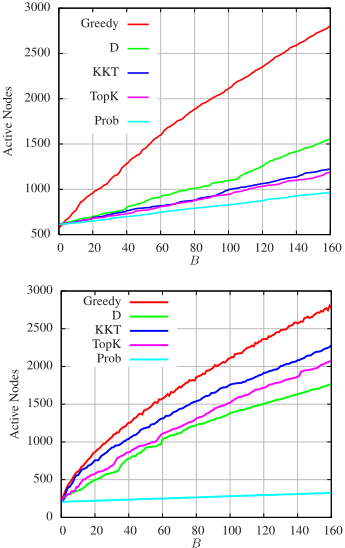
All our experiments have been performed on a computer equipped with two Intel Xeon E5-2643 CPUs (6 cores clocked at 3.4GHz) and 128GB RAM; our programs have been implemented in C++ (gcc compiler v4.8.2 with optimization level O3). We evaluate the performance of the algorithm on four types of randomly generated directed networks which exhibit many of the structural features of complex networks and on real-world graphs that are suitable for our problem, taken from KONECT [Kunegis, 2013], ArnetMiner [Arnetminer, 2015] and SNAP 3 repositories 4 . The size of the graphs are reported in Table 1. For both synthetic and real-world networks, we choose 0.1% of the nodes in V as seeds and we add up to B = 2 · |A| edges. For these experiments, the seed nodes are chosen uniformly at random. The weights on the edges in both models are generated as follows: In ICM we are assigned the probabilities to the edges according to the weighted model, i.e., for each edge (u, v), assign wuv = 1/Nv; In LTM instead we generate for each node v ∈ V a random variable ¯wv ∈ [0, 0.5] that represent the probability that v does not select any edge in the live-edge graph, then we assigned for each edge (u, v) in the graph a weight equal to 1-¯wv Nv and ¯wv 2 is assigned to a new edge. 5 As a measure of the quality of the solution, we adopt the expected number of active nodes σ(A, S). As discussed in the preliminaries, it has been proven that evaluating this function is #P-complete in general. However, by simulating the diffusion process a polynomial number of times and sampling the resulting active sets, it is possible to obtain arbitrarily good approximations to σ(A, S). We experimentally tested that 500 samples are enough to obtain a good estimation. Hence, we run 500 trial to estimate the value of σ in the algorithms and in the final solution. In Table 2, we report: σ(A, ∅) and σ(A, ∅)% that are the absolute and relative initial number of active nodes; σ(A, S) and σ(A, S)%, are the absolute and relative number of active nodes after the edge addition; the relative increment computed as I = σ(A,S)-σ(A,∅) σ(A,∅) × 100; and T, the time in seconds. The expected number of active nodes in GREEDY1 and GREEDY2 are similar, except from the time (GREEDY2 is faster), and a small difference is due to the sampling technique used to estimate ˜σ(A, S). Thus we reported the results for GREEDY2. From the table we can see that our algorithm is able to highly increase the number of activated nodes with respect to the original graph. Moreover, thanks to the reduction to LSS, the running time is small and this allows us to solve IMA in large networks. We compare GREEDY1 and GREEDY2 with the following alternatives that connect the given seed set to a set of B nodes chosen accordingly. AdamicAdar (AA): nodes with the highest Adamic-Adar [2003] index; PrefAtt (PA): nodes chosen according to the Preferential Attachment model [Bollob´as et al., 2003; Newman, 2001]; Jaccard (J): nodes with the highest Jaccard [1901] coefficient; Degree (D): nodes with the highest out-degree; Topk (TopK): nodes with the highest harmonic centrality [Boldi and Vigna, 2014]; Prob (Prob): nodes adding the edges with highest probability; Seed (KKT): nodes chosen by the greedy algorithm proposed in. [Kempe et al., 2015]; Random (R): nodes extracted uniformly at random. In Figure 1, we compare GREEDY2 with the other approaches on the Slashdot-Zoo network. Results for other networks and for GREEDY1 are similar to this case. The plots show the average number of active nodes as a function of the number of added edges. The experiments clearly show that GREEDY2 outperforms all the alternative baselines in terms of expected number of active nodes. Indeed, all the other competitive algorithms require to add a large number of edges to A in order to significantly increase the expected number of influenced nodes with respect to the initial value (B = 0), whereas our algorithm increases σ(A, S) by a greater amount with only few added edges.
3 http://snap.stanford.edu/data
4 Here we report only the results on real world networks, those on random instances can be found in the full version of the paper.
5 Note that it is unlikely that more than two edges towards the same node in V \A are added in the solution.
| G | σ(A, ∅) | σ(A, ∅)% | σ(A, S) | σ(A, S)% | I% | T |
| SE | 13.38 | 0.43 | 103.45 | 3.29 | 670.95 | 0.04 |
|---|---|---|---|---|---|---|
| TCS | 9.49 | 0.23 | 97.63 | 2.34 | 928.76 | 0.07 |
| HPC | 9.36 | 0.19 | 165.75 | 3.40 | 1670.83 | 0.07 |
| Wiki | 10.07 | 0.14 | 333.37 | 4.69 | 3257.87 | 0.12 |
| CGM | 20.34 | 0.24 | 257.62 | 3.09 | 1166.71 | 0.12 |
| CN | 22.21 | 0.24 | 397.95 | 4.22 | 1765.86 | 0.10 |
| ICM AI | 68.94 | 0.25 | 1017.82 | 3.69 | 1362.71 | 0.47 |
| Sl | 126.11 | 0.25 | 612.52 | 1.20 | 408.63 | 1.72 |
| Epi | 352.17 | 0.46 | 1230.23 | 1.62 | 249.32 | 3.25 |
| Sl-z | 570.84 | 0.72 | 3425.87 | 4.40 | 505.14 | 2.63 |
| Citeseer | 683.16 | 0.18 | 13072.36 | 3.40 | 1813.52 | 12.20 |
| 2861.20 | 0.62 | 207061.00 | 44.53 | 7136.87 | 10.23 | |
| Digg | 3848.57 | 1.38 | 14835.40 | 5.31 | 285.48 | 14.32 |
| SE | 12.40 | 0.39 | 59.45 | 1.89 | 276.88 | 0.10 |
| TCS | 8.34 | 0.20 | 51.78 | 1.24 | 430.62 | 0.13 |
| HPC | 7.91 | 0.16 | 87.98 | 1.81 | 935.87 | 0.39 |
| Wiki | 9.17 | 0.13 | 120.93 | 1.70 | 1151.57 | 1.33 |
| CGM | 16.69 | 0.20 | 128.96 | 1.55 | 525.37 | 0.29 |
| CN | 18.30 | 0.19 | 204.73 | 2.17 | 936.94 | 0.43 |
| LTM AI | 53.15 | 0.19 | 530.99 | 1.92 | 767.02 | 4.74 |
| Sl | 87.97 | 0.17 | 663.43 | 1.30 | 592.51 | 6.82 |
| Epi | 174.98 | 0.23 | 2248.09 | 2.96 | 999.34 | 37.42 |
| Sl-z | 206.35 | 0.26 | 3203.52 | 4.05 | 1160.21 | 36.48 |
| Citeseer | 623.82 | 0.16 | 5901.46 | 1.54 | 846.03 | 42.98 |
| 1673.07 | 0.36 | 127414.00 | 27.40 | 7515.56 | 13.33 | |
| Digg | 447.59 | 0.16 | 14002.80 | 5.01 | 3028.52 | 128.43 |
6 Conclusions and FutureWork
We proposed a link recommendation algorithm that, differently from other link recommenders, takes into account the amount of social influence provided by the new connections to the receiver of the recommendation. Our algorithm has a theoretical performance guarantee and, moreover, we have experimentally shown that the algorithm can be used in very large real-world networks and thus can be applied in practice.
Our algorithm aims at maximizing the amount of influence of the users that receive the recommendation. This can be used to improve the popularity of niche users and counterbalance that of famous ones. One interesting open question would be to devise a link recommender that directly considers in its objective function the balancing of social influence among users, in such a way that social biases are mitigated.
Acknowledgments
This work has been partially supported by the Italian MIUR PRIN 2017 Project ALGADIMAR "Algorithms, Games, and Digital Markets".
@inproceedings{ijcai2019p304,
  title     = {Recommending Links to Maximize the Influence in Social Networks},
  author    = {Corò, Federico and D'Angelo, Gianlorenzo and Velaj, Yllka},
  booktitle = {Proceedings of the Twenty-Eighth International Joint Conference on
               Artificial Intelligence, {IJCAI-19}},
  publisher = {International Joint Conferences on Artificial Intelligence Organization},
  editor    = {Sarit Kraus},
  pages     = {2195--2201},
  year      = {2019},
  month     = {8},
  note      = {Main track},
  doi       = {10.24963/ijcai.2019/304},
  url       = {https://doi.org/10.24963/ijcai.2019/304},
}
TY - CPAPER TI - Recommending Links to Maximize the Influence in Social Networks AU - Corò, Federico AU - D'Angelo, Gianlorenzo AU - Velaj, Yllka T2 - Proceedings of the Twenty-Eighth International Joint Conference on Artificial Intelligence, IJCAI-19 PB - International Joint Conferences on Artificial Intelligence Organization PY - 2019 SP - 2195 EP - 2201 DO - 10.24963/ijcai.2019/304 UR - https://doi.org/10.24963/ijcai.2019/304 ER -Copied
Machine-readable versions of this paper, for tools and AI agents:





