
Zero-shot Learning with Many Classes by High-rank Deep Embedding Networks
Proceedings of the Twenty-Eighth International Joint Conference on Artificial Intelligence. Main track. Pages 2428-2434.
https://doi.org/10.24963/ijcai.2019/337
Keywords
- Machine Learning: Transfer, Adaptation, Multi-task Learning
- Computer Vision: Language and Vision
- Machine Learning: Classification
Abstract
Zero-shot learning (ZSL) is a recently emerging research topic which aims to build classification models for unseen classes with knowledge from auxiliary seen classes. Though many ZSL works have shown promising results on small-scale datasets by utilizing a bilinear compatibility function, the ZSL performance on large-scale datasets with many classes (say, ImageNet) is still unsatisfactory. We argue that the bilinear compatibility function is a low-rank approximation of the true compatibility function such that it is not expressive enough especially when there are a large number of classes because of the rank limitation. To address this issue, we propose a novel approach, termed as High-rank Deep Embedding Networks (GREEN), for ZSL with many classes. In particular, we propose a feature-dependent mixture of softmaxes as the image-class compatibility function, which is a simple extension of the bilinear compatibility function, but yields much better results. It utilizes a mixture of non-linear transformations with feature-dependent latent variables to approximate the true function in a high-rank way, which makes GREEN more expressive. Experiments on several datasets including ImageNet demonstrate GREEN significantly outperforms the state-of-the-art approaches.
- [Akata et al., 2015] Zeynep Akata, Scott E. Reed, Daniel Walter, Honglak Lee, and Bernt Schiele. Evaluation of output embed- dings for fine-grained image classification. In CVPR, 2015.
- [Akata et al., 2016] Zeynep Akata, Florent Perronnin, Zaïd Har- chaoui, and Cordelia Schmid. Label-embedding for image clas- sification. IEEE Trans. Pattern Anal. Mach. Intell., 2016.
- [Bishop and others, 2006] Christopher M Bishop et al. Pattern recognition and machine learning, volume 1. Springer, New Y- ork, 2006.
- [Bishop, 1998] Christopher M Bishop. Latent variable models. In Learning in graphical models, pages 371-403. Springer, 1998.
- [Changpinyo et al., 2016] Soravit Changpinyo, Wei-Lun Chao, Bo- qing Gong, and Fei Sha. Synthesized classifiers for zero-shot learning. In 2016 IEEE Conference on Computer Vision and Pat- tern Recognition, pages 5327-5336, 2016.
- [Farhadi et al., 2009] Ali Farhadi, Ian Endres, Derek Hoiem, and David A. Forsyth. Describing objects by their attributes. In 2009 IEEE Computer Society Conference on Computer Vision and Pat- tern Recognition, pages 1778-1785, 2009.
- [Frome et al., 2013] Andrea Frome, Gregory S. Corrado, Jonathon Shlens, Samy Bengio, Jeffrey Dean, Marc'Aurelio Ranzato, and Tomas Mikolov. Devise: A deep visual-semantic embedding model. In NIPS, 2013.
- [Fu et al., 2015a] Yanwei Fu, Timothy M. Hospedales, Tao Xiang, and Shaogang Gong. Transductive multi-view zero-shot learning. IEEE Trans. Pattern Anal. Mach. Intell., 2015.
- [Fu et al., 2015b] Zhenyong Fu, Tao Xiang, Elyor Kodirov, and Shaogang Gong. Zero-shot object recognition by semantic man- ifold distance. In CVPR, 2015.
- [Guo et al., 2016] Yuchen Guo, Guiguang Ding, Xiaoming Jin, and Jianmin Wang. Transductive zero-shot recognition via shared model space learning. In AAAI, 2016.
- [Guo et al., 2017a] Yuchen Guo, Guiguang Ding, Jungong Han, and Yue Gao. Synthesizing samples for zero-shot learning. In Proceedings of the Twenty-Sixth International Joint Conference on Artificial Intelligence, pages 1774-1780, 2017. IJCAI
- [Guo et al., 2017b] Yuchen Guo, Guiguang Ding, Jungong Han, and Yue Gao. Zero-shot learning with transferred samples. IEEE TIP, 26(7):3277-3290, 2017.
- [He et al., 2016] Kaiming He, Xiangyu Zhang, Shaoqing Ren, and Jian Sun. Deep residual learning for image recognition. In CVPR, 2016.
- [Kodirov et al., 2017] Elyor Kodirov, Tao Xiang, and Shaogang Gong. Semantic autoencoder for zero-shot learning. In CVPR, 2017.
- [Lampert et al., 2014] Christoph H. Lampert, Hannes Nickisch, and Stefan Harmeling. Attribute-based classification for zero- shot visual object categorization. IEEE Trans. Pattern Anal. Mach. Intell., 36(3):453-465, 2014.
- [Mikolov et al., 2013a] Tomas Mikolov, Kai Chen, Greg Corrado, and Jeffrey Dean. Efficient estimation of word representations in vector space. ICLR Workshops, 2013.
- [Mikolov et al., 2013b] Tomas Mikolov, Ilya Sutskever, Kai Chen, Gregory S. Corrado, and Jeffrey Dean. Distributed represen- tations of words and phrases and their compositionality. In Advances in Neural Information Processing Systems 26, pages 3111-3119, 2013.
- [Norouzi et al., 2013] Mohammad Norouzi, Tomas Mikolov, Samy Bengio, Yoram Singer, Jonathon Shlens, Andrea Frome, Greg Corrado, and Jeffrey Dean. Zero-shot learning by convex combi- nation of semantic embeddings. CoRR, abs/1312.5650, 2013.
- [Patterson and Hays, 2012] Genevieve Patterson and James Hays. SUN attribute database: Discovering, annotating, and recogniz- ing scene attributes. In CVPR, 2012.
- [Romera-Paredes and Torr, 2015] Bernardino Romera-Paredes and Philip H. S. Torr. An embarrassingly simple approach to zero- shot learning. In ICML, 2015.
- [Russakovsky et al., 2015] O. Russakovsky, J. Deng, H. Su, J. Krause, S. Satheesh, S. Ma, Z.g Huang, A. Karpathy, A. Khosla, M. S. Bernstein, A. C. Berg, and Fei-Fei Li. Ima- genet large scale visual recognition challenge. IJCV, 2015.
- [Socher et al., 2013] Richard Socher, Milind Ganjoo, Christo- pher D. Manning, and Andrew Y. Ng. Zero-shot learning through cross-modal transfer. In NIPS, 2013.
- [Wah et al., 2011] Catherine Wah, Steve Branson, Peter Welinder, Pietro Perona, and Serge Belongie. The Caltech-UCSD Birds- 200-2011 Dataset. Technical Report CNS-TR-2011-001, Cali- fornia Institute of Technology, 2011.
- [Wu et al., 2018] Fan Wu, Kai Tian, Jihong Guan, and Shuigeng Zhou. Global semantic consistency for zero-shot learning. In ECCV, 2018.
- [Xian et al., 2016] Yongqin Xian, Zeynep Akata, Gaurav Sharma, Quynh N. Nguyen, Matthias Hein, and Bernt Schiele. Latent embeddings for zero-shot classification. In CVPR, 2016.
- [Xian et al., 2017] Yongqin Xian, Christoph H. Lampert, Bern- t Schiele, and Zeynep Akata. Zero-shot learning -A compre- hensive evaluation of the good, the bad and the ugly. CoRR, ab- s/1707.00600, 2017.
- [Yang et al., 2017] Zhilin Yang, Zihang Dai, Ruslan Salakhutdinov, and William W. Cohen. Breaking the softmax bottleneck: A high- rank RNN language model. In ICLR, 2017.
- [Yang et al., 2018] Zhilin Yang, Zihang Dai, Ruslan Salakhutdinov, and William W. Cohen. Breaking the softmax bottleneck: A high- rank RNN language model. In ICLR, 2018.
- [Zhang and Saligrama, 2015] Ziming Zhang and Venkatesh Saligrama. Zero-shot learning via semantic similarity embed- ding. In ICCV, 2015.
- [Zhang and Saligrama, 2016] Ziming Zhang and Venkatesh Saligrama. Zero-shot learning via joint latent similarity embedding. In CVPR, 2016.
References were extracted automatically from the PDF and may contain errors.
Full text extracted automatically from the PDF; figures, tables and equations may differ. The PDF is the version of record.
1 Introduction
The aim of zero-shot learning is to recognize concepts that are never seen during training [Xian et al., 2017]. It is very useful in real-world applications because of the following three reasons. Firstly, there are potentially unlimited concepts in practice such that it is very expensive to collect sufficient labeled samples for all of them [Lampert et al., 2014]. Secondly, new concepts emerge every data and it is almost impossible to retrain a model every time a new concept pops up. Thirdly, the objects or concepts "in the wild" follow a long-tail distribution such that many concepts have very limited visual samples for training [Changpinyo et al., 2016].
Generally speaking, ZSL can be formulated as a crossmodality matching problem equipped with a compatibility function F(x, y;W) where x ∈ Rp is the feature vector of an image such as deep features [He et al., 2016], y ∈ Rq is the feature vector of a concept such as class attributes [Farhadi et al., 2009] or word2vec representations [Socher et al., 2013], and W ∈ Rp×q is the parameter of the function F. The bilinear compatibility function defined as F(x, y;W) = xWy′ is widely utilized [Akata et al., 2016; 2015; Kodirov et al., 2017; Norouzi et al., 2013; Socher et al., 2013; Xian et al., 2016; Zhang and Saligrama, 2015]. Since there is no labeled samples for unseen classes for training, some auxiliary seen classes related to the unseen ones which have many labeled samples are utilized for training. In particular, given an image-class pair (x, y) from seen classes, the parameter W is learned with the objective that increases F(x, y;W) for a positive pair and decreases it for a negative pair. Since the seen classes and unseen classes are related (e.g., they are all animal species), the parameter W trained with seen classes can be applied to the unseen ones. Then given any image x and an class y, the compatibility can be directly computed by F(x, y;W) and the prediction of a test image x is given based on its compatibility to each unseen class, e.g., by choosing the class with the largest response.
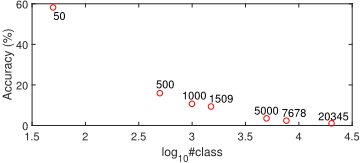
For small-scale datasets with only a few classes, such as AwA [Lampert et al., 2014] which just has 50 classes in total, bilinear compatibility function has yielded promising results, which has been demonstrated in massive number of ZSL literatures [Akata et al., 2016; Guo et al., 2017b; Kodirov et al., 2017; Zhang and Saligrama, 2015]. However, when dealing with large-scale datasets with many classes, like ImageNet [Russakovsky et al., 2015] which has thousands of classes, the performance is still unsatisfactory [Xian et al., 2017]. Since the latter is the case of real-world scenario where we wish to apply ZSL, it is necessary to investigate how to improve ZSL accuracy when there are many classes. For demonstration, we plot the current state-of-the-art ZSL accuracy w.r.t. the number of classes in the test set, as shown in Figure 1. When there are 50 test classes, the accuracy is around 60% [Changpinyo et al., 2016]. But it drops below 10% when there are more than one thousand test classes. Moreover, the test accuracy keeps decreased until it reaches less than 1%, when the test classes are increased to more than ten thousands [Xian et al., 2017].
If we regard the model learning as a function approximation problem, i.e., we try to approximate a true compatibility function F ∗ by F, the complexity of F becomes crucial. A simple model may lead to under-fitting while a complicated model may result in over-fitting [Bishop and others, 2006]. When dealing with small-scale datasets, the bilinear compatibility function seems complicated enough. However, when there are a large number of classes (say, 10 thousand), its complexity seems too low to approximate F ∗ . We argue that this is caused by the rank limitation from a matrix factorization perspective. Because the bilinear compatibility function is a (relatively) low-rank approximation, it seems too simple to handle the complicated situation when there are many classes. From this point of view, it is necessary to improve the complexity of the function to handle large-scale datasets.
On the other hand, ZSL for a large-scale dataset is different from the one for a small-scale dataset. In particular, in small datasets, it only needs to recognize coarse-grained classes like in AwA [Lampert et al., 2014], or fine-grained classes from one root category like CUB [Wah et al., 2011]. However, for a large-scale dataset like ImageNet, there are many root categories and fine-grained sub-categories, like tens of kinds of dogs and birds. In this scenario, a model has to capture macro characteristics to distinguish between root categories, such as bird and dog, and micro ones to distinguish between fine-grained classes, such as "Labrador Retriever" and "Golden Retriever". Obviously, using a simple bilinear model to handle a large-scale dataset seems unreasonable [Xian et al., 2016] such that a more expressive model is required.
The success of bilinear function for ZSL motivates us to investigate it deeper. Inspired by [Yang et al., 2018], we propose a novel approach, termed as High-rank Deep Embedding Networks (GREEN), for ZSL with many classes. Inspired by the latent variable models [Bishop, 1998], GREEN adopts a mixture of sotmaxes together with featuredependent latent variables. By the weighted combination of softmaxes, the complexity of the model is improved such that it breaks the rank limitation suffered by the bilinear model, which makes GREEN effective for ZSL with many classes from the theoretical perspective. On the other hand, the latent variables can be regarded as a coarse clustering of data which groups images with similar macro characteristics, such as views or backgrounds into one branch, followed by a softmax focusing on the micro characteristics to distinguish between them, making GREEN more powerful and flexible than the bilinear model. In summary, the contributions are below.
- We notice that the widely used bilinear compatibility function suffers from rank limitation so that it performs poorly for ZSL with many classes. We propose novel Highrank Deep Embedding Networks (GREEN) for ZSL with
- many classes. It adopts a mixture of softmaxes with featuredependent latent variables. GREEN is capable of keeping the formulation and training simple while resulting in a highcomplexity model to handle large-scale datasets.
- We develop a shallow version which utilizes given features and a deep version which can be trained in an end-to-end manner. Both versions can be trained efficiently.
- We carry out extensive experiments for ZSL with many classes, including ImageNet. The experimental results demonstrate that GREEN outperforms the state-of-the-art ZSL approaches, which validates its effectiveness.
2 Preliminaries
2.1 Notations
ZSL problem is described as follows. There are two disjoint class sets Cs = {cs1 , ..., csks } and Cu = {cu1 , ..., cuku } with Cs ∩ Cu = ∅, denoted as seen classes and unseen classes respectively. Each image is represented by an image feature vector x ∈ Rp and each class is represented by a label feature vector y ∈ Rq . There is a training set Dtr = {(xi, yi)}ns i=1 where the each class feature yi corresponds to a seen class from Cs. A compatibility function F(x, y;W) between image and class features is trained based on the training set. Then, it is applied to a test sample from unseen classes Cu in the conventional ZSL setting, or Cs ∪ Cu in the generalized ZSL setting. The classification is performed by selecting the class which has the largest compatibility to the test sample.
2.2 RelatedWorks
The bilinear compatibility function is widely utilized:
There are many representative works with it, including DEVISE [Frome et al., 2013], ALE [Akata et al., 2016], SJE [Akata et al., 2015], SAE [Kodirov et al., 2017], ESZSL [Romera-Paredes and Torr, 2015], and many other approaches [Fu et al., 2015b; 2015a; Guo et al., 2016; Zhang and Saligrama, 2016]. The basic idea is to build a cross-modality matching function between image feature space and class feature space, which can be achieved by using the labeled data in Dtr. Since the class features from Cs and Cu are from the same feature space like the word2vec space and Cs and Cu are related, e.g., they are all animal species, the function F trained with Cs can be applied to Cu, which has been demonstrated in many ZSL literatures. To learn the function F, many different loss functions are considered. For example, triplet loss [Akata et al., 2015], ranking loss [Akata et al., 2016], Euclidean loss [Romera-Paredes and Torr, 2015] and cross-entropy loss [Wu et al., 2018]. Bilinear compatibility function is shown to be simple and effective for ZSL.
There are also some other ideas for ZSL. For example, as seminal works of ZSL, DAP and IAP [Farhadi et al., 2009; Lampert et al., 2014] consider to recognize the attributes from images and compare them to the class attributes. CMT [Socher et al., 2013] embeds image features into the class feature space for distance measure. CONSE [Norouzi et al., 2013] utilizes convex combination of semantic embeddings to compute the conditional probability. SYNC [Changpinyo et al., 2016] builds synthesized classifiers based on a mapping from class feature space to a model space. SSZSL [Guo et al., 2017a] synthesizes samples based on the reconstructed distribution of unseen classes. STZSL [Guo et al., 2017b] transfers similar training samples to unseen classes based on the image-class similarity. Although they do not explicitly adopt bilinear compatibility function in Eq. (1) as the final classification model, Eq. (1) still acts as an important part in their algorithms.
3 High-rank Deep Embedding Networks
3.1 Rank Limitation
Suppose there are n images and k classes, given the parameter matrix W , we can construct an image-class compatibility matrix F ∈ Rn×k , where each element Fic = F(xi, yc;W) = xiWy′c . If the ground-truth compatibility matrix for these image-class pairs is ˜F ∈ Rn×k , we have
where X ∈ Rn×p is the image feature matrix by stacking xi and Y ∈ Rc×q is the class feature matrix by stacking yc. Interestingly, this formulation is essentially a matrix factorization problem where the matrices W, X, and Y (if learnable) are learned by some algorithms so that the factorized matrix XWY ′ can approximate ˜F as precise as possible.
Suppose the rank of F and ˜F are r and ˜ r respectively. Obviously, to precisely factorize ˜F into XWY ′ , the ranks should satisfy the condition r ≥ ˜ r or at least r is close to ˜ r. From the definition of these matrices, we can observe that r ≤ min(p, q) and ˜ r ≤ k. For a small dataset with only tens of classes, ˜ r is usually small such that the condition is always true. In this case, the bilinear compatibility function can well approximate the true function. However, for a large-scale dataset with large k, ˜ r could be very large because the real-world dataset is complicated and it is reasonable to assume the true compatibility matrix is high-rank. However, the widely used class features, such as word2vec representation [Mikolov et al., 2013a; 2013b], have only hundreds of dimensions, or even tens of dimensions. Since r ≤ q, the rank of F is much smaller than the rank of ˜F, making the approximation imprecise. Due to the rank limitation, the bilinear function seems to "underfit" datasets with many classes, yielding poor performance.
3.2 GREEN
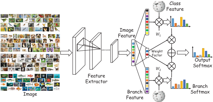
To address the issues above, in this paper we propose a novel model using a simple extension of bilinear compatibility function, termed as high-rank deep embedding networks (GREEN). The framework is summarized in Figure 2. In particular, given an image feature x, instead of utilizing the simple bilinear compatibility function in Eq. (1), we propose to use a mixture of softmaxes with feature-dependent latent variables to compute the compatibility,
where B is the number of branches and ωx,b is the featuredependent latent weight factor which controls the contribution of the b-th branch to the output, defined as follows,
where ub ∈ Rp is the weight parameter. For each branch, the branch-specific feature xb = ReLU(xVb) ∈ Rd where Vb ∈ Rp×d is the fully connected parameter, and Wb ∈ Rd×q is the compatibility parameter for the b-th branch.
One can verify F (x, yc; W) ≥ 0 and ∑c F (x, yc; W) = 1 which indicates that we can regard it as the conditional probability on each training class. Therefore we can train the model like training with conventional softmax by cross entropy loss function as follows,
Minimizing LCE is achieved by the gradient descent algorithm, which gives us the most important model parameters {ub}Bb=1 for computing the latent weight factor, {Vb}Bb=1 for computing branch-specific feature, and {Wb}Bb=1 as the compatibility parameter for each branch. With the model FG, the prediction for a test image x is given as follows,
3.3 Discussion
GREEN leads to high-rank approximation. As discussed above, bilinear function suffers from rank limitation such that it underfits the dataset which has many classes. GREEN is a simple extension of bilinear function, but results in a highrank compatibility matrix. In particular, the compatibility matrix FG produced by GREEN is as follows:
where Ωb = diag(ωx1,b, ..., ωxns ,b), Xb ∈ Rns×d is the branch-specific feature matrix by stacking training features of the b-th branch, Λb = diag(log ∑˜ c∈Cs exp(xi,bWby′˜ c ), i = 1, ..., ns), and Jns,ks is a ns × ks matrix whose elements are all 1. Obviously, FG is a non-linear combination of image features and class features by the sum-exp function. Since Λ is a diagonal matrix, the rank dG is no longer limited by the feature dimensionality p or q, making it arbitrarily high-rank. Please refer to [Yang et al., 2017] for proof. In the extreme case where B = 1, FG degenerates to F after a log transformation and a simple row-wise shift. Therefore, GREEN results in a higher-rank matrix than the bilinear model, which is able to approximate complicated datasets with many classes more precisely. Due to its improved expressiveness, we can expect GREEN to obtain better (or at least equal) results compared to the simple bilinear function.
GREEN keeps the model simple. Based on the rank limitation r ≤ min(p, q), there is a straightforward solution to problem. One can significantly increase the dimensionality of image and class features, i.e., p and q. However, when p and q get too large, the bilinear model becomes very complicated since W has p×q parameters, which is likely to overfit the training set. In addition, the number of semantic classes is potentially unlimited, it is almost impossible to keep increasing p and q when there are more classes are taken into consideration. Both issues make the model quite complicated. On the other hand, GREEN utilizes mixture of softmaxes and non-linear transformations, which is capable of approximating arbitrarily high-rank matrix, and keeping the model simple at the same time. In particularly, GREEN needs only p × b parameters to compute the feature-dependent latent weight factor, and B × p × d parameters in total. Since B is usually small (e.g., 16), the complexity is controlled. In addition, because GREEN do not suffer from rank limitation any longer, it becomes possible to reduce p and q, especially p by the branch-specific feature, to compensate for the increase of model parameters caused by the mixture structure. In this way, GREEN keeps as simple as the original bilinear compatibility model while being more expressive and powerful.
Relation to existing works. As discussed above, GREEN is an simple and effective extension of the bilinear function, which address the rank limitation problem when dealing with many classes. We also notice that there are some works considering similar mixture structure of bilinear functions. One is LATEM[Xian et al., 2016] whose compatibility function is
It utilize max operation to bring in nonlinearity. GREEN is different from LATEM in three folds. Firstly, due to the max operation, only one component contribute to the final decision in LATEM. As discussed above, with only one component, the model suffers from rank limitation. GREEN uses soft combinations such that all branches contribute to the final decision, making it more expressive. Secondly, LATEM uses triplet loss for training while GREEN directly uses softmax based cross entropy loss. Obviously, training with cross entropy loss is much easier and more efficient than with triplet loss. We can expect better performance with better optimization. Thirdly, LATEM observed the limitation of linear function but did not point out the reason. We theoretically demonstrate that the problem lies in the rank limitation and propose GREEN to effectively address it. Because of these advantages, GREEN is more powerful for ZSL with many classes.
4 Experiment
4.1 Setting
There are many widely used benchmarks for evaluating ZSL approaches. In this paper, we focus on ZSL with many classes. Therefore, many of them with only tens of classes, like AwA and aPY [Farhadi et al., 2009], are not good choices. In this paper, we consider two datasets. The first is SUN [Patterson and Hays, 2012] scene recognition dataset. It consists of 645 classes as the seen classes with 12, 900 samples for training, and 72 unseen classes with 1, 440 samples for test. The other dataset is ImageNet [Russakovsky et al., 2015] which is a really large-scale dataset with many classes. We use the widely used 1, 000 classes with about 1.3 images as the training set. There are another about 20k classes with about 14 million samples utilized as the test set. To comprehensively evaluate on ImageNet, we consider different subsets of the test set, including classes that are 2-hops (denoted as 2H, 1, 509 classes) and 3-hops (3H, 7, 678 classes) away from the 1, 000 seen classes, the most popular 500 (M500), 1k (M1K), and 5k (M5k) classes, and the least popular 500 (L500), 1k (L1K), and 5k (L5K) classes. For evaluation, we use average per-class top-1 accuracy [Xian et al., 2017]:
For each image, we use the ResNet-101 pretrained on ImageNet-1k as the feature extractor, which yields 2, 048dimensional image features. For SUN dataset, we use the provided class attributes as the class feature. Each class has a 102-dimensional attribute feature. For ImageNet dataset, we use the 500-dimensional word2vec representations for all classes [Changpinyo et al., 2016]. For fair comparison, we use the features provided by [Xian et al., 2017] as input.
| SUN | 2H | 3H | M500 | M1k | M5k | L500 | L1k | L5k | ALL | |
|---|---|---|---|---|---|---|---|---|---|---|
| CONSE [Norouzi et al., 2013] | 38.8 | 7.63 | 2.18 | 12.33 | 8.31 | 3.22 | 3.53 | 2.69 | 1.05 | 0.95 |
| CMT [Socher et al., 2013] | 39.9 | 2.88 | 0.67 | 5.10 | 3.04 | 1.04 | 1.87 | 1.08 | 0.33 | 0.29 |
| LATEM [Xian et al., 2016] | 55.3 | 5.45 | 1.32 | 10.81 | 6.63 | 1.90 | 4.53 | 2.74 | 0.76 | 0.50 |
| ALE [Akata et al., 2016] | 58.1 | 5.38 | 1.32 | 10.40 | 6.77 | 2.00 | 4.27 | 2.85 | 0.79 | 0.50 |
| DEVISE [Frome et al., 2013] | 56.5 | 5.25 | 1.29 | 10.36 | 6.68 | 1.94 | 4.23 | 2.86 | 0.78 | 0.49 |
| SJE [Akata et al., 2015] | 53.7 | 5.31 | 1.33 | 9.88 | 6.53 | 1.99 | 4.93 | 2.93 | 0.78 | 0.52 |
| ESZSL [Romera-Paredes and Torr, 2015] | 54.5 | 6.35 | 1.51 | 11.91 | 7.69 | 2.34 | 4.50 | 3.23 | 0.94 | 0.62 |
| SYNC [Changpinyo et al., 2016] | 56.3 | 9.26 | 2.29 | 15.83 | 10.75 | 3.42 | 5.83 | 3.52 | 1.26 | 0.96 |
| SAE [Kodirov et al., 2017] | 40.3 | 4.89 | 1.26 | 9.96 | 6.57 | 2.09 | 2.50 | 2.17 | 0.72 | 0.56 |
| GREEN-S | 61.2 | 10.54 | 2.41 | 17.33 | 12.51 | 4.44 | 6.60 | 5.09 | 1.61 | 1.57 |
| GREEN-D | 65.6 | 12.38 | 3.41 | 18.80 | 14.47 | 5.38 | 7.71 | 6.07 | 2.30 | 2.06 |
GREEN can take feature vectors as input like many other ZSL approaches, which can be regarded as fixing the feature extractor in Figure 2. We denote this version as GREENS(hallow). In addition, it is simple to combine GREEN with deep convolutional networks, and thus it can use raw images as input and train (finetune) the feature extractor, which is denoted as GREEN-D(eep). For both versions, we set the number of branches as B = 16. Since there are multiple branches, we can reduce the dimensionality of the branch feature xb to reduce computational burden. In particular, we set d = 256. To minimize the loss function in Eq. (5), we use mini-batch based stochastic gradient descent algorithm. The batch size is 128 and we train the model for 100k iterations. The initial learning rate is 0.01 and then 0.001 at the 70k-th iteration. For GREEN-D, we use ResNet-101 as the backbone. We implement GREEN in TensorFlow1 .
4.2 Benchmark Comparison
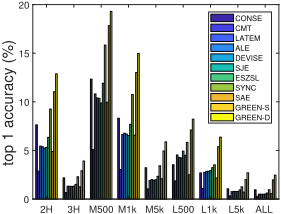
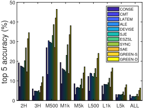
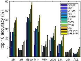
We summarize the comparison on SUN and ImageNet (including its subsets) in Table 1. In Figure 3, we show the results on ImageNet with different metrics. From the results, we can observe that GREEN outperforms the other ZSL approaches with significant margin, which demonstrates the effectiveness of GREEN for ZSL with many classes. We have the following important observations based on the results.
1 https://www.tensorflow.org/
Firstly, GREEN-S, which uses the same image features as many non-deep baseline approaches, shows observable improvement. This is a clear evidence of the superiority of GREEN framework. As discussed above, GREEN utilizes a mixture of softmaxes with feature-dependent latent weight factors to address the rank limitation problem suffered by the simple bilinear model, which is capable of approximating the true compatibility matrix in a high-rank manner. From the results, we can observe that the simple formulation of GREEN can indeed approximate the true compatibility more precisely.
Secondly, GREEN-D, which finetunes the feature extractor, improves significantly over GREEN-S. This phenomenon is reasonable since the finetuning results in better image features. However, some baseline approaches are based on deep networks too, such as CONSE and DEVISE. They do not show comparable performance. This phenomenon demonstrates that the mixture of softmaxes and the objective function of GREEN is more effective for ZSL, especially when there are many classes. In addition, SYNC is one of the best baseline approaches in all. Its nonlinear compatibility function seems work well for ZSL. However, since it is very complicated, it seems difficult to combine it with deep networks, while the simple loss function of GREEN can be combined with deep networks easily, making GREEN more powerful.
Thirdly, we show the relative improvement of GREEN-S over the best result achieved by baseline approaches. Here we can observe that the improvement becomes larger with more test classes. There are macro characteristics to distinguish between "dog" and "bird", and micro characteristics to distinguish between fine-grained classes like "Golden Retriever" and "Labrador Retriever". When there are just a few classes, one simple linear more is likely to handle both. However, when there are a large number of classes, it is unreasonable to handle them at the same time. The mixture structure of GREEN can model the hierarchical structure classes where the latent weight factors can be regarded as coarse clustering of data which distinguish between root classes and each branch focuses on fine-grained classes. The results demonstrate the superiority of GREEN for ZSL with many classes, which makes it more practical for real-world applications.
Fourthly, LATEM, which uses max operation to bring nonlinearity into compatibility function, does not perform well. As discussed above, with max operation, only one branch contributes to the final decision, which also suffers from rank limitation to some extent. GREEN uses soft combinations using all branches, making it more expressive, which seems more reasonable and suffers less from the rank limitation.
4.3 The Effect of Mixture
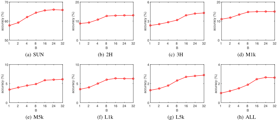
To further verify the effectiveness of GREEN, we conduct another experiment, which change the number of branches, i.e., B, and evaluate the performance of GREEN-D. When B = 1, GREEN-D degenerates to the simple bilinear model. The results w.r.t. B are shown in Figure 4. We can observe that the performance increases significantly with larger B, which shows the importance of the mixture of softmaxes. When there are many classes, it is unreasonable to handle them by a simple bilinear model. With more branches in the mixture, the model can focuses on more aspects of data, such as different background or views, and then capture the micro information in each branch. Besides, although the sum-exp function can theoretically result in arbitrarily high rank, the rank of the generated compatibility function in practice is still limited by the complexity of the model due to the existence of model regularization. With more branches in the mixture, the model is more expressive, leading to higher-rank approximation.
5 Conclusion
In this paper we focus on ZSL with many classes. In particular, we notice that the widely used bilinear compatibility function works well on small-scale datasets, but fails in largescale datasets with many classes like ImageNet. We argue that this is due to the rank limitation problem based on a matrix factorization perspective. To address this issue, we propose a novel approach, termed as High-rank Deep Embedding Networks (GREEN). GREEN utilizes a mixture of softmaxes as the image-class compatibility function, which is a simple extension of bilinear function, but is able to approximate the true function in a high-rank manner by a mixture of nonlinear transformations with feature-dependent latent variables. GREEN is very simple and expressive. It can be combined with deep networks as well. Extensive experiments on benchmarks including ImageNet demonstrate GREEN significantly outperforms the state-of-the-arts for ZSL with many classes.
Acknowledgements
This work was supported by the National Key R&D Program of China (No. 2018YFC0807500), National Natural Science Foundation of China (No. 61571269), National Postdoctoral Program for Innovative Talents (No. BX20180172), and the China Postdoctoral Science Foundation (No. 2018M640131). Email: yuchen.w.guo@gmail.com. Corresponding author: Guiguang Ding, dinggg@tsinghua.edu.cn.
@inproceedings{ijcai2019p337,
  title     = {Zero-shot Learning with Many Classes by High-rank Deep Embedding Networks},
  author    = {Guo, Yuchen and Ding, Guiguang and Han, Jungong and Shao, Hang and Lou, Xin and Dai, Qionghai},
  booktitle = {Proceedings of the Twenty-Eighth International Joint Conference on
               Artificial Intelligence, {IJCAI-19}},
  publisher = {International Joint Conferences on Artificial Intelligence Organization},
  editor    = {Sarit Kraus},
  pages     = {2428--2434},
  year      = {2019},
  month     = {8},
  note      = {Main track},
  doi       = {10.24963/ijcai.2019/337},
  url       = {https://doi.org/10.24963/ijcai.2019/337},
}
TY - CPAPER TI - Zero-shot Learning with Many Classes by High-rank Deep Embedding Networks AU - Guo, Yuchen AU - Ding, Guiguang AU - Han, Jungong AU - Shao, Hang AU - Lou, Xin AU - Dai, Qionghai T2 - Proceedings of the Twenty-Eighth International Joint Conference on Artificial Intelligence, IJCAI-19 PB - International Joint Conferences on Artificial Intelligence Organization PY - 2019 SP - 2428 EP - 2434 DO - 10.24963/ijcai.2019/337 UR - https://doi.org/10.24963/ijcai.2019/337 ER -Copied
Machine-readable versions of this paper, for tools and AI agents:





