
Robust Low-Tubal-Rank Tensor Completion via Convex Optimization
Proceedings of the Twenty-Eighth International Joint Conference on Artificial Intelligence. Main track. Pages 2649-2655.
https://doi.org/10.24963/ijcai.2019/368
Keywords
- Machine Learning: Learning Theory
- Machine Learning: Unsupervised Learning
- Computer Vision: Statistical Methods and Machine Learning
- Machine Learning Applications: Applications of Unsupervised Learning
Abstract
This paper considers the problem of recovering multidimensional array, in particular third-order tensor, from a random subset of its arbitrarily corrupted entries. Our study is based on a recently proposed algebraic framework in which the tensor-SVD is introduced to capture the low-tubal-rank structure in tensor. We analyze the performance of a convex program, which minimizes a weighted combination of the tensor nuclear norm, a convex surrogate for the tensor tubal rank, and the tensor l1 norm. We prove that under certain incoherence conditions, this program can recover the tensor exactly with overwhelming probability, provided that its tubal rank is not too large and that the corruptions are reasonably sparse. The number of required observations is order optimal (up to a logarithm factor) when comparing with the degrees of freedom of the low-tubal-rank tensor. Numerical experiments verify our theoretical results and real-world applications demonstrate the effectiveness of our algorithm.
- [Braman, 2010] Karen Braman. Third-order tensors as linear operators on a space of matrices. Linear Algebra & Its Applications, 433(7):1241-1253, 2010.
- [Candés and Recht, 2009] Emmanuel J. Candés and Ben- jamin Recht. Exact matrix completion via convex op- timization. Foundations of Computational Mathematics, 9(6):717-772, 2009.
- [Candés et al., 2011] Emmanuel J. Candés, Xiaodong Li, Yi Ma, and John Wright. Robust principal component analysis? Journal of the ACM, 58(3):1-73, May 2011.
- [Chen, 2013] Yudong Chen. Incoherence-optimal matrix completion. IEEE TIT, 61(5):2909-2923, 2013.
- [Dabov et al., 2007] Kostadin Dabov, Alessandro Foi, Vladimir Katkovnik, and Karen Egiazarian. Image restoration by sparse 3D transform-domain collaborative filtering. IEEE TIP, 16(8):2080-2095, August 2007.
- [Gandy et al., 2011] Silvia Gandy, Benjamin Recht, and Isao Yamada. Tensor completion and low-n-rank ten- sor recovery via convex optimization. Inverse Problems, 27(2):025010, 2011.
- [Gu et al., 2014] Quanquan Gu, Huan Gui, and Jiawei Han. Robust tensor decomposition with gross corruption. In Proceedings of the 27th Advances in Neural Information Processing Systems, pages 1422-1430, 2014.
- [Huang et al., 2014] Bo Huang, Cun Mu, Donald Goldfarb, and John Wright. Provable low-rank tensor recovery. Optimization-Online, page 4252, 2014.
- [Jain and Oh, 2014] Prateek Jain and Sewoong Oh. Prov- able tensor factorization with missing data. In NIPS, pages 1431-1439, 2014.
- [Karlsson et al., 2016] Lars Karlsson, Daniel Kressner, and André Uschmajew. Parallel algorithms for tensor com- pletion in the CP format. Parallel Comput., 57:222-234, September 2016.
- [Kilmer and Martin, 2011] Misha E. Kilmer and Carla D. Martin. Factorization strategies for third-order tensors. Linear Algebra and its Applications, 435(3):641-658, 2011.
- [Kilmer et al., 2013] Misha E. Kilmer, Karen Braman, Ning Hao, and Randy C. Hoover. Third-order tensors as oper- ators on matrices: a theoretical and computational frame- work with applications in imaging. SIAM Journal on Mat. Analy. & App., 34(1):148-172, 2013.
- [Kokaram, 2004] Anil C. Kokaram. On missing data treat- ment for degraded video and film archives: A survey and a new bayesian approach. IEEE TIP, 13(3):397-415, March 2004.
- [Kolda and Bader, 2009] Tamara G. Kolda and Brett W. Bader. Tensor decompositions and applications. SIAM Review, 51(3):455-500, 2009.
- [Li, 2013] Xiaodong Li. Compressed sensing and matrix completion with constant proportion of corruptions. Con- structive Approximation, 37(1):73-99, 2013.
- [Liu et al., 2013] Ji Liu, Przemyslaw Musialski, Peter Wonka, and Jieping Ye. Tensor completion for estimating missing values in visual data. IEEE T PAMI, 35(1):208- 220, 2013.
- [Lu et al., 2016] Canyi Lu, Jiashi Feng, Yudong Chen, Liu Wei, and Shuicheng Yan. Tensor robust principal compo- nent analysis: Exact recovery of corrupted low-rank ten- sors via convex optimization. In CVPR, pages 5249-5257, 2016.
- [Lu et al., 2018] Canyi Lu, Jiashi Feng, Yudong Chen, Liu Wei, Zhouchen Lin, and Shuicheng Yan. Tensor robust principal component analysis with a new tensor nuclear norm. arXiv:1804.03728, 2018.
- [Martin et al., 2001] David R. Martin, Charless Fowlkes, Doron Tal, and Jitendra Malik. A database of human seg- mented natural images and application to evaluating seg- mentation algorithms and measuring ecological statistics. ICCV, 2(11):416-423, 2001.
- [Martin et al., 2013] Carla D. Martin, Richard Shafer, and Betsy Larue. An order-p tensor factorization with applica- tions in imaging. SIAM Journal on Scientific Computing, 35(1):A474-A490, 2013.
- [Mu et al., 2013] Cun Mu, Huang Bo, John Wright, and Donald Goldfarb. Square deal: Lower bounds and im- proved relaxations for tensor recovery. In ICML, pages 73-81, 2013.
- [Shah et al., 2015] Parikshit Shah, Nikhil Rao, and Gongguo Tang. Sparse and low-rank tensor decomposition. In NIPS, pages 2548-2556, 2015.
- [Shang et al., 2014] Fanhua Shang, Yuanyuan Liu, James Cheng, and Hong Cheng. Robust principal component analysis with missing data. In CIKM, pages 1149-1158, November 2014.
- [Subrahmanyam et al., 2010] Gorthi R.K.S. Subrahmanyam, Ambasamudram N. Rajagopalan, and Rangarajan Ar- avind. Recursive framework for joint inpainting and de- noising of photographic films. Journal of the Optical So- ciety of America A, 27(5):1091-1099, 2010.
- [Tomioka et al., 2010] Ryota Tomioka, Kohei Hayashi, and Hisashi Kashima. Estimation of low-rank tensors via con- vex optimization. arXiv:1010.0789, 2010.
- [Tomioka et al., 2011] Ryota Tomioka, Taiji Suzuki, Kohei Hayashi, and Hisashi Kashima. Statistical performance of convex tensor decomposition. In NIPS, pages 972-980, 2011.
- [Wright et al., 2013] John Wright, Arvind Ganesh, Kerui Min, and Yi Ma. Compressive principal component pur- suit. Information and Inference, 2(1):32-68, 2013.
- [Zhang and Aeron, 2017] Zemin Zhang and Shuchin Aeron. Exact tensor completion using t-SVD. IEEE TSP, 65(6):1511-1526, 2017.
- [Zhang et al., 2014] Zemin Zhang, Gregory Ely, Shuchin Aeron, Ning Hao, and Misha Kilmer. Novel methods for multilinear data completion and de-noising based on tensor-SVD. In CVPR, pages 3842-3849, 2014.
References were extracted automatically from the PDF and may contain errors.
Full text extracted automatically from the PDF; figures, tables and equations may differ. The PDF is the version of record.
1 Introduction
Real data, such as electroencephalography (EEG), video, and color image, is usually multidimensional in nature. Tensorbased modeling is a proper choice for such data because it is capable of taking full advantage of the underlying multilinear structures to provide better understanding and higher accuracy. In many applications, multidimensional data is probably incomplete or corrupted owing to various unpredictable or unavoidable factors. The tremendous demand for clean data leads to increasing interest in tensor sampling, estimation and recovery during the last decade.
The strategies and their performance for tensor sampling and recovery rely heavily on the low-rank decomposition used to reveal the intrinsic structure in the multidimensional data. For matrix (second-order tensor) data, its rank defined by means of the smallest number of rank-one matrix decomposition, can be easily obtained via singular value decomposition (SVD). The nuclear norm has been shown to be the convex envelope of matrix rank over a unit ball of spectral norm. Under some mild assumptions, efficient techniques based on convex programming to minimize the nuclear norm can recover the low-rank matrices accurately (or perhaps exactly) from severely compressive [Wright et al., 2013], incomplete [Cand´es and Recht, 2009; Chen, 2013], or corrupted observations [Cand´es et al., 2011; Li, 2013].
∗This work was conducted when the authors were with the Department of Mathematics, Hong Kong Baptist University.
†Corresponding Author
Unlike the matrix case, several definitions of tensor rank and their convex relaxations can be found in literature. However, each has its own drawbacks. The CANDECOMP/PARAFAC (CP) decomposition [Kolda and Bader, 2009] compresses a tensor as the sum of rank-one outer products. The minimal number of such decomposition is defined as the CP rank, which is NP-hard to compute in general [Kolda and Bader, 2009]. Although efforts [Jain and Oh, 2014; Shah et al., 2015; Karlsson et al., 2016] have been made to recover low-CP-rank tensor in some special cases, it still remains computationally intractable to determine the CPrank or its best convex approximation. The Tucker rank of a tensor is a vector whose entries are the ranks of unfolding matrices along each mode respectively [Kolda and Bader, 2009]. Inspired by the relation between matrix rank and nuclear norm, Liu et al. proposed the Sum of Nuclear Norms (SNN), which is the (weighted) sum of the nuclear norms of unfolding matrices, as a convex relaxation for Tucker rank. The effectiveness of this tractable measure has been successfully validated in both theoretical analyses [Tomioka et al., 2011; Gu et al., 2014] and practical settings (see, e.g., [Tomioka et al., 2010; Gandy et al., 2011] and reference therein). Considering that the approximation may be substantially suboptimal in certain situations, Mu et al. further designed a better (but still sub-optimal) convex surrogate for tensor rank through a more balanced matricization.
The tensor-product and associated algebraic constructs introduced for third [Kilmer and Martin, 2011] and higher order tensors [Martin et al., 2013], provide a new framework in which we can obtain a SVD-like factorization named the tensor-SVD (t-SVD) [Kilmer and Martin, 2011; Martin et al., 2013], and derive a notion of tensor rank referred to as the tubal rank [Kilmer et al., 2013]. Using this new algebraic framework, Zhang and Aeron and Lu et al. gave sufficient conditions for convex programming to succeed in exact recovery of low-tubal-rank tensors from incomplete and grossly corrupted observations respectively.
This paper considers a more challenging problem, namely, recovering a low-rank tensor from a small fraction of its entries, part of which are even arbitrarily corrupted. In essence, this problem is tensor-based generalization of robust matrix completion (RMC) [Li, 2013; Shang et al., 2014]. This is why we call it robust tensor completion (RTC) hereafter. Leveraging on the t-SVD algebraic framework, we study the performance of a convex optimization model and provide recovery guarantee. Specifically, we show that when certain tensor incoherence conditions are satisfied, the convex program can exactly recover the low-tubal-rank tensor with high probability, provided that the tubal rank is not too large and that the corruptions are reasonably sparse. The sampling complexity is order optimal (up to a logarithm factor) when comparing with the degrees of freedom of the tensor.
We are aware that the RTC problem has been theoretically examined in [Huang et al., 2014]. Our study departs from that work on several fronts. First, the t-SVD algebraic framework, in which third-order tensors are treated as linear operators over matrices oriented laterally [Kilmer et al., 2013; Braman, 2010], is quite different from the multilinear algebraic setup for Tucker decomposition. Besides, the tubal rank and tensor nuclear norm differ seriously from the Tucker rank and its convex relaxation SNN. Consequently, the recovery theory established in [Huang et al., 2014] is not directly comparable to our result.
2 Notations and Preliminaries
We first go over some notations. In this paper, tensors are denoted by boldface Euler letters, e.g., A, matrices by boldface capital letters, e.g., A, vectors by boldface lowercase letters, e.g., a, and scalars by lowercase letters, e.g., a. The field of real number and complex number are denoted as R and C, respectively. We denote ⌊n⌋ as the nearest integer less than or equal to n and ⌈n⌉ as the one greater than or equal to n.
For a third-order tensor A ∈ Rn1×n2×n3 , we denote its (i, j, k)-th entry as Aijk and denote its i-th horizontal, lateral and frontal slice using the MATLAB notation A(i, :, :), A(: , i, :) andA(:, :, i), respectively. For simplicity, the front slice A(:, :, i) is denoted compactly as A(i) . A(i, j, :) denotes a tubal fiber oriented into the board obtained by fixing the first two indices and varying the third. Moreover, a tensor tube of size 1 × 1 × n3 is denoted as ˙a and a tensor column of size n1 × 1 × n3 is denoted as˚b.
For a vector v ∈ Cn , the ℓ2-norm is ‖v‖2 = √∑i |vi|2 . The inner product of A and B in Cn1×n2 is given by 〈A,B〉 = Tr(AH B), where AH denotes the conjugate transpose of A and Tr(·) denotes the matrix trace. The spectral norm of a matrix A ∈ Cn1×n2 is denoted as ‖A‖ = maxi σi(A), where σi(A)'s are the singular values of A. The matrix nuclear norm is ‖A‖∗ = ∑i σi(A). The inner product of A and B in Cn1×n2×n3 is defined as 〈A,B〉 = ∑n3 i=1 〈A(i) ,B(i) 〉. For any A ∈ Cn1×n2×n3 , the complex conjugate of A is denoted as conj(A) which takes the complex conjugate of all entries of A. We denote the ℓ1-norm as ‖A‖1 = ∑ijk |Aijk|, the infinity norm as ‖A‖∞ = maxijk |Aijk| and the Frobenius norm as ‖A‖F = √∑ijk |Aijk|2 . These norms reduce to the corresponding vector or matrix norms if A is a vector or a matrix.
For A ∈ Rn1×n2×n3 , using the MATLAB command fft, we denote ¯ A ∈ Cn1×n2×n3 as the result of Fast Fourier Transformation (FFT) of A along the third dimension, i.e., ¯ A = fft(A, [], 3). In the same fashion, we can compute A from ¯ A using the inverse FFT, i.e., A = ifft( ¯ A, [], 3). Furthermore, we define the block circulant matrix of A as
and the following operators
Definition 1 (t-product) [Kilmer and Martin, 2011] The tproduct A∗ B of A ∈ Rn1×n4×n3 and B ∈ Rn4×n2×n3 is a tensor C ∈ Rn1×n2×n3 ,
For the frontal slices of ¯ A, we have
Using the above property, we can compute t-product by a more efficient way (see [Lu et al., 2018, Algorithm 1]).
Definition 2 (Conjugate transpose) [Kilmer and Martin, 2011] The conjugate transpose of a tensor A ∈ Rn1×n2×n3 is the tensor AH ∈ Rn2×n1×n3 obtained by conjugate transposing each of the frontal slice and then reversing the order of transposed frontal slices 2 through n3.
Definition 3 (Identity tensor) [Kilmer and Martin, 2011] The identity tensor I ∈ Rn×n×n3 is defined to be a tensor whose first frontal slice is the n×n identity matrix and whose other frontal slices are zero matrices.
Definition 4 (Orthogonal tensor) [Kilmer and Martin, 2011] A tensor Q ∈ Rn×n×n3 is orthogonal if it satisfies
Definition 5 (f-diagonal tensor) [Kilmer and Martin, 2011] A tensor A is called f-diagonal if each frontal slice A(i) is a diagonal matrix.
Definition 6 (t-SVD) [Kilmer and Martin, 2011; Lu et al., 2018] For A ∈ Rn1×n2×n3 , the t-SVD of A is given by
where U ∈ Rn1×n1×n3 and V ∈ Rn2×n2×n3 are orthogonal tensors, and S ∈ Rn1×n2×n3 is a f-diagonal tensor.
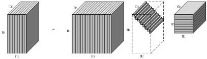
The entries of the first frontal slice S(:; :; 1) are called the singular values of the tensor A [Lu et al., 2018]. Figure 1 illustrates the t-SVD for a n1 ×n2 ×n3 tensor. This factorization can be obtained by computing matrix SVDs in the Fourier domain. This idea was proposed first in [Kilmer and Martin, 2011] and later some related works [Kilmer et al., 2013; Zhang and Aeron, 2017], but the way for computing U and V cannot guarantee that they are real tensors. The study [Lu et al., 2018] uses property (1) to construct U and V, which leads to a more efficient way for computing t-SVD (see [Lu et al., 2018, Algorithm 2]), and thus fixes this issue. It is only required to run ⌈ n3+1 2 ⌉ matrix SVDs while the number is n3 for the original method [Kilmer and Martin, 2011].
Definition 7 (Tensor tubal rank) [Lu et al., 2018] For A ∈ Rn1×n2×n3 , the tensor tubal rank, denoted as rankt(A), is defined as the number of nonzero singular values of S, where S is from the t-SVD of A = U ∗ S ∗ V H . We can write
For A ∈ Rn1×n2×n3 with tubal rank r, it has the skinny tSVD, i.e., A = U ∗ S ∗ U H where U ∈ Rn1×r×n3 , S ∈ Rr×r×n3 , and V ∈ Rn2×r×n3 such that U H ∗ U = I and V H ∗ V = I. The skinny t-SVD will be used in this paper.
There are some connections between tensor tubal rank and other tensor ranks. First, suppose the Tucker rank of A be (rank(A(1)), rank(A(2)), rank(A(3))), where A(i) is the ith mode matricization of A, and we have rankt(A) ≤ min(rank(A(1)), rank(A(2))). This indicates that a tensor with low Tucker rank also has low tubal rank. Moreover, let the CP decomposition of A be A = ∑ri=1 a(1) i ◦a(2) i ◦a(3) i , where ◦ denotes the outer product. Then ¯ A = ∑ri=1 a(1) i ◦ a(2) i ◦ ¯a(3) i , where ¯a(3) i = fft(a(3) i ). This implies that each frontal slice of ¯ A is the sum of r rank-one matrices and ¯ A has CP rank at most r. Therefore, the tubal rank of A is not larger than r. In a word, the low-tubal-rank assumption is weaker than the low-Tucker-rank and low-CP-rank assumptions.
Definition 8 (Tensor nuclear norm) [Lu et al., 2018] Let A = U∗S∗V H be the t-SVD of A ∈ Rn1×n2×n3 . The tensor nuclear norm of A is defined as the sum of the tensor singular values, i.e., ‖A‖∗ = ∑ri=1 S(i, i, 1), where r = rankt(A).
The above definition of tensor nuclear norm (TNN) is equivalent to that given in [Lu et al., 2016]. Indeed,
Definition 9 (Tensor spectral norm) [Lu et al., 2016] The tensor spectral norm of A ∈ Rn1×n2×n3 , denoted as ‖A‖, is defined as ‖A‖ = ‖bcirc(A)‖ = maxi ‖ ¯A(i) ‖.
It has been shown that TNN is the dual norm of the tensor spectral norm, and vice versa [Zhang et al., 2014]. If we define the tensor average rank as ranka(A) = 1 n3 rank(bcirc(A)), then the convex envelope of the tensor average rank is the tensor nuclear norm within the set {A|‖A‖ ≤ 1} [Lu et al., 2018]. We would like to emphasize that the above definition of TNN is different from the one in [Zhang and Aeron, 2017] due to the factor 1 n3 and this factor is crucial in our theoretical analysis.
3 Exact Recovery Guarantee
Let us consider the RTC problem formally. Suppose we are given a third-order tensor L0 having low tubal rank and corrupted by a sparse term E0. Here, both L0 and E0 are of arbitrary magnitude. We do not know the tubal rank of L0. Also we have no idea about the locations of the nonzero entries of E0, not even how many there are. Can we recover L0 accurately (perhaps even exactly) and efficiently from an observed subset of the noisy data X = L0 + E0? 1
Mathematically, the problem can be represented by
where λ is a penalty parameter and PΩ is a linear projection such that the entries in the set Ω are given while the remaining entries are missing. The optimization problem (2) is generally NP-hard due to the discrete nature of the tubal rank and the ℓ0 pseudo-norm. Replacing these two terms by their convex surrogates, namely, tensor nuclear norm and ℓ1-norm respectively, leads to the following convex optimization problem
Our model (3) is equivalent to the following tensor completion (TC) problem when there is no corruption, i.e., E = 0,
and reduces to the tensor robust principal component analysis (TRPCA) problem when Ω is the entire set of indices,
3.1 Tensor Incoherence Conditions
As discussed in [Huang et al., 2014; Lu et al., 2016; Zhang and Aeron, 2017; Lu et al., 2018], exact recovery is hopeless if most entries of X are equal to zero. When X is both lowrank and sparse (e.g., X111 = 1 and zeros everywhere else), we are not able to identify the low-rank tensor L0. To make the problem meaningful, we need some tensor incoherence conditions on L0. We denote˚ei as the tensor column basis, which is a tensor of size n1 ×1×n3 with its (i, 1, 1)-th entry equaling 1 and the rest equaling 0. We also define the tensor tube basis ˙ek, which is a tensor of size 1 × 1 × n3 with its (1, 1, k)-th entry equaling 1 and the rest equaling 0.
1 In this situation, it is impossible to exactly recover E0 (some of its entries are simply not observed!), unless the observed set is identical to the support of E0.
Definition 10 (Tensor Incoherence Conditions) Assume that rankt(L0) = r and its skinny t-SVD is L0 = U∗S∗V H . L0 is said to satisfy the tensor incoherence conditions with parameter µ0 > 0 if
and
The incoherence conditions (6)-(8) reduce to the regular matrix incoherence conditions [Cand´es and Recht, 2009; Cand´es et al., 2011; Li, 2013] when n3 = 1. According to [Chen, 2013], we name (6) and (7) tensor standard incoherence conditions, and (8) tensor joint incoherence condition. Zhang and Aeron indicate that the joint incoherence condition (8) is unnecessary for tensor completion, while we get the same conclusion in an alternative way. However, this incoherence condition is indispensable for obtaining exact solution to the TRPCA and RTC problems, as shown in our analysis 2 . Another concern arises if the corruption term E0 has low tubal rank. This can be avoided by assuming that the support of E0 is distributed uniformly at random.
3.2 Main Results
Now we present our main results. For convenience, we denote n(1) = max(n1, n2) and n(2) = min(n1, n2).
Theorem 1 Suppose L0 ∈ Rn1×n2×n3 obeys (6)-(8), and the observation set Ω is uniformly distributed among all sets of cardinality m = ρn1n2n3. Also suppose that each observed entry is independently corrupted with probability γ. Then, there exist universal constants c1, c2 > 0 such that with probability at least 1-c1(n(1)n3)-c2 , the recovery of L0 with λ = 1/√ρn(1)n3 is exact, provided that
where cr and cγ are two positive constants.
The theorem tells us that the target tensor L0 whose singular vectors U(:, i, :) and V(:, j, :) are reasonably spread, can be exactly recovered with probability nearly one from a subset of its entries even if they are arbitrarily corrupted. All we require is that the tubal rank of the tensor L0 is not too large, to be exact, on the order of n(2)/(µ0(log(n(1)n3))2 ) and the corruption term E0 is sufficiently sparse. We would like to emphasize that the only "random distribution" in our assumptions concerns the locations of the nonzero entries of E0, but not on their magnitudes or signs. Another remarkable fact is that there is no tuning parameter in our model.
2 The proof of Theorem 1, the optimization algorithm to solve (3), and additional experimental results are given in the longer version of this paper: http://www.math.hkbu.edu.hk/∼mng/qiang-mng.pdf
The recovery guarantees for problems (4) and (5) are naturally implied by Theorem 1 as in the following corollaries Corollary 1 Suppose L0 ∈ Rn1×n2×n3 obeys (6) and (7) and m entries of L0 are observed with locations sampled uniformly at random, then there exist universal constants c0, c1, c2 > 0 such that if
L0 is the unique minimizer to (4) with probability at east 1c1(n(1)n3)-c2 .
Corollary 2 Suppose L0 ∈ Rn1×n2×n3 obeys (6)-(8) and E0 has support uniformly distributed with probability γ. Then, there exist universal constants c1, c2 > 0 such that with probability at least 1-c1(n(1)n3)-c2 , (L0, E0) is the unique minimizer to (5) with λ = 1/√n(1)n3, provided that
where cr and cγ are two positive constants.
It is worth pointing out that the theoretical results given here can be easily extended to the case of pth-order tensors with p ≥ 3, by exploiting the higher-order t-SVD algebraic framework [Martin et al., 2013].
3.3 Connections with PriorWorks
Recall that the t-product for third-order tensors and the tubal nuclear norm reduce to the standard matrix multiplication and the matrix nuclear norm respectively when n3 = 1. In this sense, Theorem 1.3 in [Li, 2013] can be viewed as a special case of Theorem 1 in this paper.
The two works [Zhang and Aeron, 2017; Lu et al., 2018] are the most similar to our study. However, they simply focus on the TC and TRPCA problems, which are both special cases of our model. Corollary 2 seems slightly different from Theorem 4.1 in [Lu et al., 2018], but they are actually in good agreement with each other. Note that our incoherence parameter µ0 and the incoherence parameter µ given in [Lu et al., 2018] have the relationship µ0 = µ n3 . Substituting the equation into (6)-(8) and (11), we obtain the identical results.
The number of observed entries m required by Corollary 1 is O(rn(1)n3(log(n(1)n3))2 ). For a n1 × n2 × n3 tensor with tubal rank r, its degrees of freedom is O(r(n1 +n2)n3). Therefore, such rate is order optimal (up to a logarithmic factor). The similar results have been observed in the matrix cases [Cand´es and Recht, 2009; Chen, 2013].
4 Experiments
We conduct a series of experiments to demonstrate the validity of our theorem, and show possible applications of our model and algorithm. As suggested by Theorem 1, the parameter λ is set to be λ = 1/√ρn(1)n3 in all the experiments unless otherwise specified. For practical problems, it is possible to further improve the performance by turning λ cautiously. Nevertheless, the default value is often a good rule of thumb. We employ the standard alternating direction method of multipliers (ADMM) algorithm to solve (3).
| r = 0.05n, ρ = 0.9, γ = 0.1 | r = 0.1n, ρ = 0.8, γ = 0.2 | ||||||
|---|---|---|---|---|---|---|---|
| n | r | rankt(L) | ‖L-L0‖F ‖L0‖F | n | r | rankt(L) | ‖L-L0‖F ‖L0‖F |
| 100 | 5 | 5 | 1.68×10⁻¹⁰ | 100 | 10 | 10 | 8.53 × 10⁻¹⁰ |
| 200 | 10 | 10 | 5.25×10⁻¹² | 200 | 20 | 20 | 1.13 × 10⁻¹¹ |
| 300 | 15 | 15 | 4.80×10⁻¹² | 300 | 30 | 30 | 2.26 × 10⁻¹² |
4.1 Synthetic Tensor Recovery
Validity of Exact Recovery
We first verify the correct recovery phenomenon of Theorem 1 by synthetic problems. For simplicity, we consider the tensors of size n×n×n with varying dimension n = 100, 200 and 300. We generate the clean tensor L0 = P ∗W with tubal rank rankt(L0) = r, where the entries of P ∈ Rn×r×n and W ∈ Rr×n×n are independently sampled from a standard Gaussian distribution N(0, 1). In addition, a fraction γ of its entries are uniformly corrupted by additive i.i.d. noise from a standard Gaussian distribution N(0, 1) at random. Finally, we randomly choose a percentage ρ of the noisy tensor entries as our observations.
We test on two cases and summarize the results in Table 1. We set r = 0.05n, γ = 0.1 and ρ = 0.9 for the first scenario, and choose a more challenging setting with r = 0.1n, γ = 0.2 and ρ = 0.8 for the second scenario. It is clear to see that our method gives the correct rank estimation of L0 and the negligible relative error ‖L - L0‖F/‖L0‖F in all cases. These results verify the exact recovery phenomenon as claimed in Theorem 1 pretty well.
Phase Transition
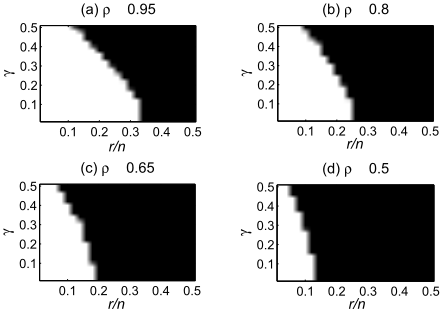
To further corroborate our theoretical results, we check the recovery ability of our algorithm as a function of tubal rank r, fractions of gross corruptions γ and proportion of observed entries ρ. The data are generated by the above-mentioned strategy, where the data size n = 100. We set ρ to be different specified values, and vary r and γ to empirically investigate the probability of recovery success. For each pair (r, γ), we simulate 10 test instances and declare a trial to be successful if the recovered tensor L satisfies ‖L-L0‖F /‖L0‖F ≤ 10-3 . Figure 2 reports the fraction of perfect recovery for each pair (black = 0% and white = 100%). We see clearly that there exists a big region in which the recovery is correct for all the cases. Moreover, the larger the percentage of missing values is, the smaller the region of correct recovery becomes.
4.2 Natural Image Restoration
It is well known that the real color images can be well approximated by low-rank matrices on the three channels independently. If a color image is treated as a third-order tensor with each channel corresponding to a frontal slice, then it can be well approximated by a tensor of low tubal rank [Liu et al., 2013; Lu et al., 2016]. In this experiment, we focus on noisy image completion. Unlike the traditional problems of image inpainting and image denoising, this problem aims to simultaneously fill the missing pixels and remove the noise in an image. One typical example is the restoration of archived photographs and films [Kokaram, 2004; Subrahmanyam et al., 2010]. In this case, it is necessary to deal with corruptions and missing values jointly.
We download 50 color images at random from the Berkeley Segmentation Database (BSD) [Martin et al., 2001]. For each image, we randomly set γ pixels corrupted with Gaussian noise N(0, σ), and choose ρ entries to be observed. We compare our algorithm with several approaches for low-rank matrix or tensor recovery, including RPCA [Cand´es et al., 2011], RMC [Shang et al., 2014], SNN [Huang et al., 2014], and TRPCA [Lu et al., 2016]. For RPCA and RMC, we apply them on each channel independently with λ = 1/√n(1). For SNN, we find that its performance is not satisfactory when the parameters λi's are set to the default values [Huang et al., 2014]. As suggested by [Lu et al., 2016], we empirically set λ1 = λ2 = 15 and λ3 = 1.5 which make SNN work fine for most images. We run TRPCA with λ = 1/√n(1)n3. For a comprehensive comparison, we also test BM3D 3 [Dabov et al., 2007] on the BSD image set, which is usually referred to as the representative of state-of-the-art algorithms for image restoration. Considering that BM3D is originally proposed for image denoising, we further enhance it with the scheme of "completion + denoising", which means that we first fill the missing pixels without considering the noise and then apply BM3D to the intermediate result. Here, HaLRTC 4 [Liu et al., 2013] and TNNM [Zhang et al., 2014] are used in the completion step and the corresponding methods are denoted by BM3D+ and BM3D++, respectively.
We consider two different situations in which ρ is set to be 0.9 and 0.7 respectively, and change γ from 0.01 to 0.03 for each case. Table 2 gives the results in terms of average Peak Signal-to-Noise Ratio (PSNR) and Structural Similarity index (SSIM) when σ = 30. The best results is in bold text and the second one is underlined. Our algorithm yields the best quantitative results for all the cases, significantly better than the runner-up sometimes. The performance of TRPCA
3 http://www.cs.tut.fi/∼foi/GCF-BM3D/index.html
4 http://www.cs.rochester.edu/u/jliu/publications.html
| ρ = 0.9 | ρ = 0.7 | |||||||||||
|---|---|---|---|---|---|---|---|---|---|---|---|---|
| γ = 0.1 | γ = 0.2 | γ = 0.3 | γ = 0.1 | γ = 0.2 | γ = 0.3 | |||||||
| PSNR | SSIM | PSNR | SSIM | PSNR | SSIM | PSNR | SSIM | PSNR | SSIM | PSNR | SSIM | |
| RPCA | 27.67 | 0.8535 | 27.30 | 0.8367 | 26.88 | 0.8122 | 21.69 | 0.5609 | 20.62 | 0.4744 | 19.64 | 0.4081 |
| RMC | 28.11 | 0.8552 | 27.82 | 0.8423 | 27.53 | 0.8276 | 26.33 | 0.7865 | 26.09 | 0.7736 | 25.84 | 0.7599 |
| TRPCA | 32.31 | 0.9457 | 31.59 | 0.9278 | 30.91 | 0.9037 | 29.25 | 0.8608 | 28.69 | 0.8209 | 28.06 | 0.7678 |
| BM3D | 28.31 | 0.8008 | 28.25 | 0.8002 | 28.18 | 0.7994 | 20.91 | 0.3392 | 20.80 | 0.3311 | 20.70 | 0.3234 |
| BM3D+ | 30.72 | 0.8289 | 30.51 | 0.8245 | 30.28 | 0.8203 | 29.75 | 0.8060 | 29.45 | 0.7993 | 29.18 | 0.7935 |
| BM3D++ | 30.94 | 0.8338 | 30.74 | 0.8297 | 30.52 | 0.8257 | 30.42 | 0.8221 | 30.11 | 0.8152 | 29.82 | 0.8093 |
| SNN | 30.14 | 0.9128 | 29.60 | 0.8972 | 29.11 | 0.8797 | 27.75 | 0.8426 | 27.35 | 0.8248 | 26.97 | 0.8063 |
| RTC | 33.03 | 0.9566 | 32.10 | 0.9400 | 31.27 | 0.9185 | 31.30 | 0.9296 | 30.58 | 0.9091 | 29.91 | 0.8831 |
is comparable to our algorithm when ρ = 0.9, but it deteriorates dramatically as ρ and γ become larger. BM3D is not able to achieve acceptable results, especially when the fraction of missing pixels is relatively high, since it considers removing the noise from the images purely. With an additional completion step, BM3D+ and BM3D++ exhibit remarkably improved performance. Three tensor-based methods, TRPCA, SNN and RTC, perform much better than two matrixbased approaches, RPCA and RMC. The reason is that RPCA and RMC, which conduct the matrix recovery on each channel independently, are incapable of exploiting the information across channels, while the tensor-based methods can take the advantage of the multi-channel structure. We also see that our quantitative results are much better than those obtained by SNN, which verifies that the t-SVD algebraic framework is more suitable for natural image processing compared with the traditional multilinear algebraic setup.
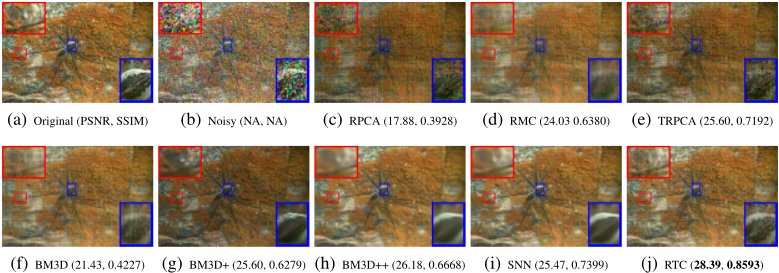
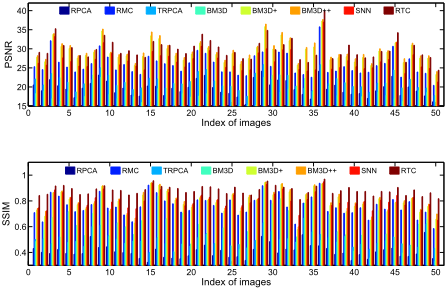
In Figure 4, we give the results obtained by various methods on all 50 images when ρ = 0.7 and γ = 0.3. Our algorithm outperforms the other methods quantitatively for most images. From the example in Figure 3, we see that our recovered images contain slightly sharper edges and fewer artifacts, exhibited in the enlarged views of the corresponding areas in red and blue boxes.
5 Conclusions
In this work, we conduct a rigourous study for the RTC problem which aims to learn a low-tubal-rank tensor from partial observations that are arbitrarily corrupted. Our study rests heavily on recently proposed t-SVD algebraic framework, in which we can define the tubal rank and tensor nuclear norm for tensors. Equipped with the new definitions, we show that one can exactly recover a third-order tensor having low tubal rank with high probability and establish a theoretical bound for exact recovery when using a convex optimization algorithm. Numerical experiments verify our theoretical analysis and the real-world applications demonstrate the superiority of our method over other existing approaches. Considering that real data routinely lies in thousands or even billions of dimensions, the computational cost of our method may become expensive. We desire to develop fast algorithms for low-tubalrank tensor recovery and will explore this important direction in our future work.
Acknowledgements
This work is supported in part by the Hong Kong RGC GRF projects 12306616, 12200317 and 12300218.
@inproceedings{ijcai2019p368,
  title     = {Robust Low-Tubal-Rank Tensor Completion via Convex Optimization},
  author    = {Jiang, Qiang and Ng, Michael},
  booktitle = {Proceedings of the Twenty-Eighth International Joint Conference on
               Artificial Intelligence, {IJCAI-19}},
  publisher = {International Joint Conferences on Artificial Intelligence Organization},
  editor    = {Sarit Kraus},
  pages     = {2649--2655},
  year      = {2019},
  month     = {8},
  note      = {Main track},
  doi       = {10.24963/ijcai.2019/368},
  url       = {https://doi.org/10.24963/ijcai.2019/368},
}
TY - CPAPER TI - Robust Low-Tubal-Rank Tensor Completion via Convex Optimization AU - Jiang, Qiang AU - Ng, Michael T2 - Proceedings of the Twenty-Eighth International Joint Conference on Artificial Intelligence, IJCAI-19 PB - International Joint Conferences on Artificial Intelligence Organization PY - 2019 SP - 2649 EP - 2655 DO - 10.24963/ijcai.2019/368 UR - https://doi.org/10.24963/ijcai.2019/368 ER -Copied
Machine-readable versions of this paper, for tools and AI agents:





