
Graph and Autoencoder Based Feature Extraction for Zero-shot Learning
Proceedings of the Twenty-Eighth International Joint Conference on Artificial Intelligence. Main track. Pages 3038-3044.
https://doi.org/10.24963/ijcai.2019/421
Keywords
- Machine Learning: Dimensionality Reduction and Manifold Learning
- Machine Learning: Classification
Abstract
Zero-shot learning (ZSL) aims to build models to recognize novel visual categories that have no associated labelled training samples. The basic framework is to transfer knowledge from seen classes to unseen classes by learning the visual-semantic embedding. However, most of approaches do not preserve the underlying sub-manifold of samples in the embedding space. In addition, whether the mapping can precisely reconstruct the original visual feature is not investigated in-depth. In order to solve these problems, we formulate a novel framework named Graph and Autoencoder Based Feature Extraction (GAFE) to seek a low-rank mapping to preserve the sub-manifold of samples. Taking the encoder-decoder paradigm, the encoder part learns a mapping from the visual feature to the semantic space, while decoder part reconstructs the original features with the learned mapping. In addition, a graph is constructed to guarantee the learned mapping can preserve the local intrinsic structure of the data. To this end, an L21 norm sparsity constraint is imposed on the mapping to identify features relevant to the target domain. Extensive experiments on five attribute datasets demonstrate the effectiveness of the proposed model.
- [Akata et al., 2015] Zeynep Akata, Scott E Reed, Daniel J Walter, Honglak Lee, and Bernt Schiele. Evaluation of output embeddings for fine-grained image classification. In CVPR, pages 2927-2936, 2015.
- [Akata et al., 2016] Zeynep Akata, Florent Perronnin, Zaid Harchaoui, and Cordelia Schmid. Label-embedding for image classification. IEEE transactions on pattern analy- sis and machine intelligence, 38(7):1425-1438, 2016.
- [Annadani and Biswas, 2018] Yashas Annadani and Soma Biswas. Preserving semantic relations for zero-shot learn- ing. In CVPR, pages 7603-7612, 2018.
- [Bartels and Stewart, 1972] Richard H. Bartels and George W Stewart. Solution of the matrix equation ax+ xb= c [f4]. Communications of the ACM, 15(9):820- 826, 1972.
- [Boyd et al., 2011] Stephen Boyd, Neal Parikh, Eric Chu, Borja Peleato, and Jonathan Eckstein. Distributed opti- mization and statistical learning via the alternating direc- tion method of multipliers. Foundations and Trends in Ma- chine Learning, 3(1):1-122, 2011.
- [Candès et al., 2011] Emmanuel J Candès, Xiaodong Li, Y- i Ma, and John Wright. Robust principal component anal- ysis? Journal of the ACM (JACM), 58(3):11, 2011.
- [Changpinyo et al., 2016] Soravit Changpinyo, Wei-Lun Chao, Boqing Gong, and Fei Sha. Synthesized classifiers for zero-shot learning. In CVPR, pages 5327-5336, 2016.
- [Chen et al., 2018] Long Chen, Hanwang Zhang, Jun Xiao, Wei Liu, and Shihfu Chang. Zero-shot visual recog- nition using semantics-preserving adversarial embedding networks. In CVPR, pages 1043-1052, 2018.
- [Der Maaten and Hinton, 2008] Laurens Van Der Maaten and Geoffrey E Hinton. Visualizing data using t-sne. Jour- nal of Machine Learning Research, 9:2579-2605, 2008.
- [Farhadi et al., 2009] Ali Farhadi, Ian Endres, Derek Hoiem, and David Forsyth. Describing objects by their attributes. In CVPR, pages 1778-1785, 2009.
- [Frome et al., 2013] Andrea Frome, Greg S Corrado, Jon Shlens, Samy Bengio, Jeff Dean, Tomas Mikolov, et al. Devise: A deep visual-semantic embedding model. In NeurIPS, pages 2121-2129, 2013.
- [Fu et al., 2015] Yanwei Fu, Timothy M Hospedales, Tao X- iang, and Shaogang Gong. Transductive multi-view zero- shot learning. IEEE transactions on pattern analysis and machine intelligence, 37(11):2332-2345, 2015.
- [He et al., 2003] Xiaofei He, Shuicheng Yan, Yuxiao Hu, and Hongjiang Zhang. Learning a locality preserving sub- space for visual recognition. In ICCV, pages 385-392, 2003.
- [He et al., 2016] Kaiming He, Xiangyu Zhang, Shaoqing Ren, and Jian Sun. Deep residual learning for image recog- nition. In CVPR, pages 770-778, 2016.
- [Kodirov et al., 2017] Elyor Kodirov, Tao Xiang, and Shao- gang Gong. Semantic autoencoder for zero-shot learning. In CVPR, pages 4447-4456, 2017.
- [Lampert et al., 2014] Christoph H Lampert, Hannes Nick- isch, and Stefan Harmeling. Attribute-based classification for zero-shot visual object categorization. IEEE Trans- actions on Pattern Analysis and Machine Intelligence, 36(3):453-465, 2014.
- [Li et al., 2019] Jin Li, Xuguang Lan, Yang Liu, Le Wang, and Nanning Zheng. Compressing unknown images with product quantizer for efficient zero-shot classification. In CVPR, 2019.
- [Liu et al., 2018a] Shichen Liu, Mingsheng Long, Jianmin Wang, and Michael I Jordan. Generalized zero-shot learn- ing with deep calibration network. In NeurIPS, pages 2009-2019, 2018.
- [Liu et al., 2018b] Yang Liu, Quanxue Gao, Jin Li, Jungong Han, and Ling Shao. Zero shot learning via low-rank em- bedded semantic autoencoder. In IJCAI, pages 2490-2496, 2018. IJCAI
- [Liu et al., 2019] Jinlu Liu, Xirong Li, and Gang Yang. Cross-class sample synthesis for zero-shot learning. In B- MVC, 2019. Nie et al., 2010] Feiping Nie, Heng Huang, Xiao Cai, and Chris H Q Ding. Efficient and robust feature selection via joint l2,1-norms minimization. In NeurIPS, pages 1813- 1821, 2010.
- [Norouzi et al., 2014] Mohammad Norouzi, Tomas Mikolov, Samy Bengio, Yoram Singer, Jonathon Shlens, Andrea Frome, Greg S Corrado, and Jeffrey Dean. Zero-shot learning by convex combination of semantic embeddings. In ICLR, 2014.
- [Palatucci et al., 2009] Mark Palatucci, Dean Pomerleau, Geoffrey E Hinton, and Tom M Mitchell. Zero-shot learn- ing with semantic output codes. In NeurIPS, pages 1410- 1418, 2009.
- [Patterson et al., 2014] Genevieve Patterson, Chen Xu, Hang Su, and James Hays. The sun attribute database: Beyond categories for deeper scene understanding. International Journal of Computer Vision, 108(1-2):59-81, 2014.
- [Romera-Paredes and Torr, 2015] Bernardino Romera- Paredes and Philip Torr. An embarrassingly simple approach to zero-shot learning. In ICML, pages 2152- 2161, 2015.
- [Socher et al., 2013] Richard Socher, Milind Ganjoo, Christopher D Manning, and Andrew Ng. Zero-shot learning through cross-modal transfer. In NeurIPS, pages 935-943, 2013.
- [Verma and Rai, 2017] Vinay Kumar Verma and Piyush Rai. A simple exponential family framework for zero-shot learning. In ECML, pages 792-808, 2017.
- [Welinder et al., 2010] P. Welinder, S. Branson, T. Mita, C. Wah, F. Schroff, S. Belongie, and P. Perona. Caltech- ucsd birds 200. Technical Report CNS-TR-2010-001, Cal- ifornia Institute of Technology, 2010.
- [Wu et al., 2019] Gengshen Wu, Jungong Han, Yuchen Guo, Li Liu, Guiguang Ding, Qiang Ni, and Ling Shao. Unsu- pervised deep video hashing via balanced code for large- scale video retrieval. IEEE Transactions on Image Pro- cessing, 28(4):1993-2007, 2019.
- [Xian et al., 2016] Yongqin Xian, Zeynep Akata, Gaurav Sharma, Quynh Nguyen, Matthias Hein, and Bern- t Schiele. Latent embeddings for zero-shot classification. In CVPR, pages 69-77, 2016.
- [Xian et al., 2018] Yongqin Xian, Christoph H Lampert, Bernt Schiele, and Zeynep Akata. Zero-shot learning - a comprehensive evaluation of the good, the bad and the ugly. IEEE Transactions on Pattern Analysis and Machine Intelligence, pages 1-1, 2018.
- [Zhang and Koniusz, 2018] Hongguang Zhang and Piotr Ko- niusz. Zero-shot kernel learning. In CVPR, pages 7670- 7679, 2018.
- [Zhang and Saligrama, 2015] Ziming Zhang and Venkatesh Saligrama. Zero-shot learning via semantic similarity em- bedding. In ICCV, pages 4166-4174, 2015.
- [Zhu et al., 2014] Xiangxin Zhu, Dragomir Anguelov, and Deva Ramanan. Capturing long-tail distributions of object subcategories. In CVPR, pages 915-922, 2014.
References were extracted automatically from the PDF and may contain errors.
Full text extracted automatically from the PDF; figures, tables and equations may differ. The PDF is the version of record.
1 Introduction
Image classification has made huge progress in recent years. With the emergence of large-scale databases, some supervised deep learning approaches show their great advantages in recognizing objects. Such methods generally train a model by hundreds of samples collected from each category and can only recognize a fixed number of classes. However, obtaining a large number of labeled samples is difficult and time consuming. In addition, the numbers of samples often follow a long-tailed distribution [Zhu et al., 2014] and it is usually impossible to collect sufficient samples for some rare categories.
∗Contact Author: Q. Gao. (qxgao@xidian.edu.cn)
Zero-shot learning (ZSL) [Palatucci et al., 2009] is designed to identify categories that have no labeled samples during the training phase with the aid of seen classes and semantic information, which is inspired by the process of human recognizing new objects. For example, even if a child has never seen a panda, if the child is told that the panda looks like a bear (seen classes) with black and white blocks (semantic information), he or she can recognize the panda correctly. In other words, ZSL primarily transfers learned knowledge from seen classes to unseen classes by establishing the relationship between seen and unseen classes during the training phase. In particular, one classic approach is to learn the mapping from the visual feature space to the semantic space during the training phase, and then use this mapping to project test samples into the semantic space during the testing phase [Akata et al., 2016]. In this case, the ZSL problem becomes a traditional classification problem, which can be achieved by common classification methods, such as the nearest neighbour (NN) method.
Most methods only learn the mapping from the visual feature space to the semantic space, but do not consider the reconstruction of visual features. This can lead to the domain shift problem [Fu et al., 2015] that adversely affects the final classification results. An effective semantic autoencoder (SAE) [Kodirov et al., 2017] is proposed to solve the problem by adding the reconstruction constraint on the representation of visual features. However, SAE does not guarantee that the learned projection can preserve the underlying sub-manifold of the samples. For example, in the visual space, the horse and the zebra are similar and the blue whale looks more like a dolphin than a horse or a zebra. Thus, the distance between the horse and the zebra should be close in the visual space. We hope such a local structure can be preserved in the semantic space as well (See Figure 1). In the meantime, we hope the projected data have a low-rank structure, which can be achieved by minimizing the nuclear norm regularization [Cand`es et al., 2011]. Moreover, L21-norm regularization is proved to be an effective method for feature selection across all samples with joint sparsity [Nie et al., 2010]. Inspired by these three points, we propose a framework named Graph and Autoencoder Based Feature Extraction method (GAFE) to learn a low-rank embedding to preserve the local structure of the data and thus has more discriminating power.
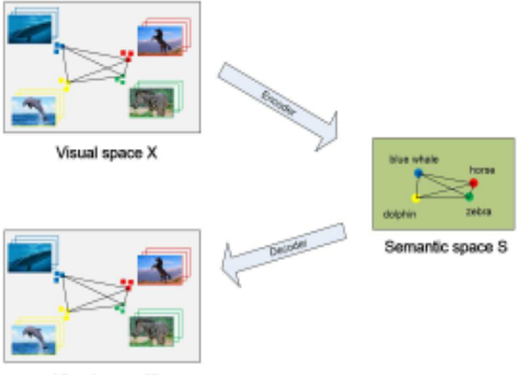
The novelty of the proposed model lies in three aspects: (1) The graph is constructed to guarantee the learned projection can preserve the local intrinsic structure of the projected data, which allows the model to have more discriminating power. (2) The shared discriminative features across unseen and seen classes can be captured by the low-rank embedding space. (3) The L21-norm regularization can help to select representative features that are more conducive to classification. We perform experiments on five popular datasets and excellent results demonstrate the effectiveness of the proposed model.
2 RelatedWorks
ZSL aims to recognize unseen classes with no training samples by transferring knowledge from seen classes with abundant training samples. The semantic space is used to associate the seen and unseen classes. There are various semantic representations available, such as attributes, word vector and text description. Many experiments show that the attribute is a valid semantic representation for ZSL [Akata et al., 2015], which indicates the intrinsic characteristic (e.g., has wings) of each class or instance. In this paper, we use attributes as semantic representations of classes.
Based on semantic embedding of class prototypes, existing ZSL models can be generally categorized as four groups: (1) Bayesian models. The Bayesian formulation is used to learn embedding models with the prior knowledge of each type of attribute. For example, DAP and IAP [Lampert et al., 2014] first learn per-attribute classifiers using supervised learning methods and then carry out recognition with Bayesian formulation. (2) Semantic embedding. Semantic embedding aims to learn the mapping from the visual feature space to the semantic space with different semantic representations. ALE [Akata et al., 2016] is an effective model and takes attribute-based classification as a label-embedding problem by minimizing the loss function between the label and image embedding. SAE [Kodirov et al., 2017] can effectively solve the projection domain shift problem by adding the reconstruction constraint on the representation of visual features. Motivated by SAE, many models are proposed recently and show good performance[Liu et al., 2018b]. (3) Embedding into common spaces. Different from the semantic embedding, a common intermediate space can be exploited to learn the relationship between the visual feature space and the semantic space. SJE [Akata et al., 2015] aims to learn a common space including multiple semantics, such as text, attributes and hierarchical relationships. Other methods such as [Romera-Paredes and Torr, 2015; Li et al., 2019] also aim to learn common spaces in different ways. (4) Deep embedding. ZSL can also be implemented by deep learning methods. DeViSE [Frome et al., 2013] is first proposed to solve the problem by pretraining deep language and visual models. In recent years, more and more deep learning networks [Norouzi et al., 2014; Wu et al., 2019] have been proposed to solve ZSL tasks.
3 Approach
3.1 ProblemDefinition
Suppose there are n labeled samples with c seen classes {X, S,Y} and nu unlabeled samples with cu unseen classes {Xu,Su,Yu}, where X ∈ Rd×n and Xu ∈ Rd×nu are d-dimensional visual features, while the corresponding labels are Y and Yu respectively. The seen and unseen classes are disjoint, i.e., Y ∩ Yu = ∅. S ∈ Rk×n and Su ∈ Rk×nu are k-dimensional semantic representations of samples in the seen and unseen classes. The ZSL task aims to learn a classifier f : Xu → Yu, where classes of testing data Xu are unseen in the training phrase.
3.2 The ProposedModel
As explained earlier in the introduction, the SAE model [Kodirov et al., 2017] does not guarantee that the learned projection can preserve the underlying manifold of the samples. Then we have the following formulation:
(1)
where W is the projection from visual feature space to semantic space and L is the Laplacian matrix. L is defined as L = P - Q, where Q is the similarity matrix and P is the degree matrix, which is a diagonal matrix whose i-th diagonal element is ∑j qij . α and β are weighting coefficients that balance these terms.
According to Eq. (1), our motivation can be explained as follows: (1) The first and the second terms indicate the SAE model, which can be described as a bidirectional loss between the feature and semantic representations of samples. (2) The third term is the graph regularization based on the Locality Preserving Projection (LPP) [He et al., 2003], which constructs a graph and preserves the local structure of data manifold. It allows the model to have more discriminating power. (3) The fourth term is the low-rank constraint based on nuclear-norm, which integrates the merits of both semantic representation learning and low-rank discriminative embedding. In this way, the shared discriminative features across unseen and seen classes can be captured by the low-rank embedding space. (4) The last term is the L21-norm regularization for feature selection, which can help to select representative features that are more conducive to classification.
3.3 Optimization Algorithm
In order to solve the objective function, we rewrite the Eq. (1) as follows:
Eq. (2) can be solved effectively by Alternating Direction Method of Multipliers (ADMM) method [Boyd et al., 2011]. The augmented Lagrangian function of Eq. (2) is formulated by
where Y1 is the estimate of the Lagrange multiplier and 〈·, ·〉 is defined as the inner product operator. µ is a positive scalar. It is not easy to minimize the Larangian function directly. An effective method to solve Eq. (3) is the alternating direction method by optimizing each variable alternatively while fixing others. Then the optimization problem can be solved by optimizing several subproblems as follows.
Step 1: Update B while fixing the other variables. Problem (3) is reduced to solve problem (4):
where M = 2S+µWX-Y1 2+µ , Ωα/(2+µ) (M) = USα/(2+µ) (∑)VT , U ∑ VT is the singular value decomposition (SVD) of M and the scale shrinkage operator [Cand`es et al., 2011] is defined as Sε (Z) = sign (z) · max (|z| - ε, 0).
Step 2: Update Wwhile fixing the other variables. In this
Algorithm 1 : ADMM algorithm for GAFE
Input: Data matrix X, semantic matrix S Parameter: µmax = 106 , ρ = 1.1, ε = 10-3 , α and β Output: W
- 1: Initialize B=W=Y1= 0, and µ = 0.1.
- 2: while ‖B-WX‖∞ < ε do
- 3: Update B using Eq. (4).
- 4: UpdateWusing Eq. (6) by Bartels-Stewart method.
- 5: Update Y1 and the parameter µ using Eq. (9) and Eq. (10).
- 6: end while
- 7: returnW
case, Eq. (3) becomes
Taking a derivative of Eq. (5) and set it zero, we have
It is worth noting that the derivative of ‖W‖2,1 is defined as
where D is a diagonal matrix with the i-th diagonal element as
where wi is defined as the i-th column of W.
Eq. (6) is a Sylvester equation which can be solved efficiently by the Bartels-Stewart algorithm [Bartels and Stewart, 1972].
Step 3: Update Y1 and the parameter µ. They are updated by Eq. (9) and Eq. (10)
where ρ > 1 and µmax are constants.
The procedure of solving Eq. (2) is listed in Algorithm 1.
The classification process can be performed in the visual feature space or the semantic space. In this paper, we use the first method. That is, when the projection matrix W is well learned, we use WT to project prototypes of unseen classes Su to the visual feature space. Then the label of the testing sample Xiu can be classified by Nearest Neighbour (NN) search with the help of following equation:
where Xiu and Sju are the i-th column of Xu and j-th column of Su. And d (·, ·) represents the distance between two vectors. In this paper, we use cosine distance to calculate the similarity.
| Dataset | Attribute dim | s/u classes | s/u samples |
|---|---|---|---|
| SUN | 102 | 645/72 | 10320/1440 |
| CUB | 312 | 150/50 | 7057/2967 |
| AWA1 | 85 | 40/10 | 19832/5685 |
| AwA2 | 85 | 40/10 | 23527/7913 |
| aPY | 64 | 20/12 | 5932/7924 |
4 Experiments
4.1 Datasets
The statistics of the five benchmark datasets are shown in Table 1.
SUN Attribute (SUN) [Patterson et al., 2014] is a finegrained dataset, containing 14,340 samples from 717 categories and 102 attributes. According to [Lampert et al., 2014], 645 classes are used for training and others for testing.
CUB-200-2011 Birds (CUB) [Welinder et al., 2010] is a fine-grained dataset. It has 11,788 samples from 200 different types of birds and the number of attributes is 312. Following [Welinder et al., 2010], the training and testing classes are 150 and 50 respectively.
Animals with Attributes 1 (AWA1) [Lampert et al., 2014] is a coarse-grained dataset, containing 30,475 visual features and 85 class-level attributes. The number of seen and unseen classes are 40 and 10 respectively.
Animals with Attributes 2 (AWA2) [Xian et al., 2018] consists of 37,322 visual features and 85 class-level attributes. Similarly, 40/10 classes are used for training/testing and all of the 50 categories are the same as AWA1 dataset.
A Pascal and Yahoo (aPY) [Farhadi et al., 2009] is a small scale coarse-grained dataset, containing 15,339 samples and 64 semantic features, in which 20 classes are used for training and 12 others for testing.
To make fair comparisons, the class semantics and image features provided by [Xian et al., 2018] are used in our experiments. Specifically, the visual features are extracted by the 101-layered ResNet [He et al., 2016] and the attribute vectors are utilized as the class semantics.
4.2 EvaluationMetrics and ComparisonMethods
The average per-class Top-1 accuracy is used for the evaluation criteria, which is formulated by
where Υ and ‖Υ‖ are defined as the set of categories and number of categories respectively. In other words, Υ consists of all the unseen classes, i.e. the testing classes.
The generalized zero-shot learning (GZSL) is another evaluation criteria, whose search space at testing time is not restricted to only testing categories (Υts ), but consists of the training ones (Υtr ). In this case, we can compute acc (Υts )
| Type | Method | SUN | CUB | AWA1 | AWA2 | aPY |
|---|---|---|---|---|---|---|
| Deep | DEVISE | 56.5 | 52.0 | 54.2 | 59.7 | 39.8 |
| CONSE | 38.8 | 34.3 | 45.6 | 44.5 | 26.9 | |
| CMT | 39.9 | 34.6 | 39.5 | 37.9 | 28.0 | |
| SP- AEN | 59.2 | 55.4 | - | 58.5 | 24.1 | |
| PSR | 61.4 | 56.0 | - | 63.8 | 38.4 | |
| DCN | 61.8 | 56.2 | 65.2 | - | 43.6 | |
| CCSS | 56.8 | 44.1 | 56.3 | 63.7 | 35.5 | |
| Shallow | DAP | 39.9 | 40.0 | 44.1 | 46.1 | 33.8 |
| IAP | 19.4 | 24.0 | 35.9 | 35.9 | 36.6 | |
| SSE | 51.5 | 43.9 | 60.1 | 61.0 | 34.0 | |
| LATEM | 55.3 | 49.3 | 55.1 | 55.8 | 35.2 | |
| ALE | 58.1 | 54.9 | 59.9 | 62.5 | 39.7 | |
| SJE | 53.7 | 53.9 | 65.6 | 61.9 | 32.9 | |
| ESZSL | 54.5 | 53.9 | 58.2 | 58.6 | 38.3 | |
| SYNC | 56.3 | 55.6 | 54.0 | 46.6 | 23.9 | |
| SAE | 59.7 | 50.9 | 53.0 | 66.0 | 35.1 | |
| GAFE | 62.2 | 52.6 | 67.9 | 67.4 | 44.3 |
and acc (Υtr ) by Eq. (12). In addition, the harmonic mean can be computed as follows
In the experiment, we compare the proposed model with many competitive or representative methods, including shallow methods DAP [Lampert et al., 2014], IAP [Lampert et al., 2014], SSE [Zhang and Saligrama, 2015], SJE [Akata et al., 2015], ESZSL [Romera-Paredes and Torr, 2015], LatEm [Xian et al., 2016], ALE [Akata et al., 2016], SYNC [Changpinyo et al., 2016], SAE [Kodirov et al., 2017], GFZSL [Verma and Rai, 2017], ZSKL [Zhang and Koniusz, 2018] and deep methods DeViSE [Frome et al., 2013], CMT [Socher et al., 2013], CONSE [Norouzi et al., 2014], SP-AEN [Chen et al., 2018], PSR [Annadani and Biswas, 2018], DCN [Liu et al., 2018a], CCSS [Liu et al., 2019].
4.3 Zero-Shot Learning Classification
We compare our proposed GAFE with other methods under the same experimental conditions in Table 2.
It can be seen from Table 2, our proposed GAFE outperforms the other models on all datasets except the CUB dataset. We owe the success of GAFE to the maintenance of the manifold structure. Especially on the AWA1 and aPY datasets, the accuracy has been significantly improved compared with SAE. As a fine-grained dataset, most classes are very similar in CUB, so less discriminative manifold structure could be obtained in the visual space by the GAFE. While PSR or DCN model learns more complicated classifiers to enhance the discriminative property in the visual space.
4.4 Generalized Zero-Shot Learning Classification
To demonstrate the effectiveness of the proposed model, we also apply our method to the GZSL task.
It can be seen from Table 3, most compared approaches get low accuracy on the acc (Υts ) and H because of overfitting the seen classes, while the GAFE method achieves more balanced results between the unseen and seen classes especially on AWA1, AWA2 and aPY datasets and is comparable to the best approach on the other datasets. In addition, our proposed model achieves better results than SAE in all datasets. Specifically, on the AWA1 dataset, the GAFE increases 7.2% and 8.4% in acc (Υts ) and H than the existing best method respectively, which demonstrates the maintenance of manifold structure and selection of effective features benefit the GZSL task.
4.5 Parameter Settings and Convergence Analysis
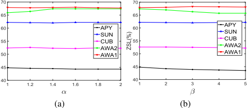
Our proposed model has two free parameters: α and β (see Eq. (1)). Figure 2 shows the variation of the best results for these two parameters over a small range. From the parameter analysis on α (see Figure 2 (a)), our GAFE achieves the best result when α = 1.4 on the AWA2 dataset while the value of α approaches one on other four datasets. From the parameter analysis on β (see Figure 2 (b)), our GAFE achieves the best result when β = 1 on aPY and AWA2 datasets while the value of β approaches three other three datasets. Empirically, α can be set to 1 < α < 1.4, while β varies from 1 to 3.
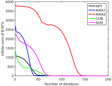
The convergence curve of all datasets is shown in Figure 3. It is clear that our algorithm converges within only 160 steps on the AWA2 dataset and 80 steps on other four datasets. The good convergence guarantees the reliability of our model.
4.6 Visualized Results
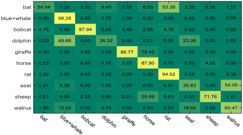
We further provide some visualized results for the proposed method. Figure 4 shows the confusion matrices of unseen classes on the AWA2 dataset. For each confusion matrix, the column represents the ground truth and the row denotes the predicted results.
According to Figure 4, it is clear that the proposed model GAFE can identify most of unseen categories, except "bat", "dolphin", "seal" on the AWA2 dataset. Considering the fact that no samples from these unseen classes are used to train the model, it strongly supports the superiority of GAFE for effective zero-shot learning.
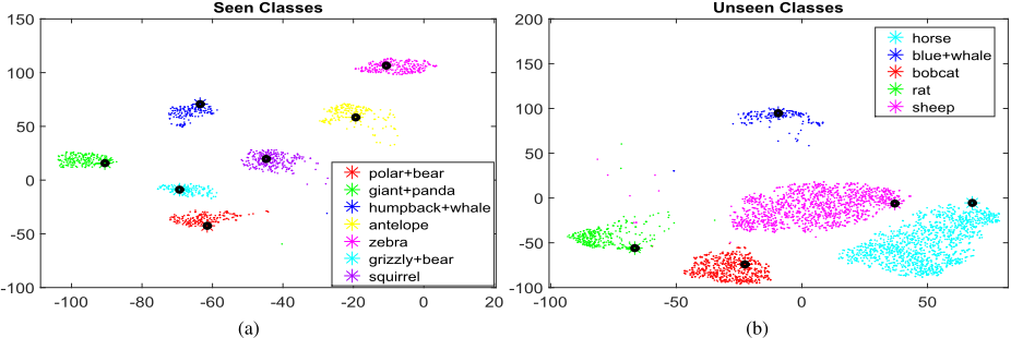
The prototype of each class usually locate near the samples that belongs to the corresponding class. In order to check whether the prototypes are properly learned, we visualize the prototypes and corresponding samples in the semantic space with the help of t-SNE method [Der Maaten and Hinton, 2008]. We select 7 seen classes and 5 unseen classes from the AWA2 dataset. Figure 5 shows the visualization results.
Although the testing classes are unseen in the training phrase, Figure 5 shows that most samples locate near the prototypes of the corresponding classes. It demonstrates our model can learn a proper projection from the visual feature space to the semantic space.
5 Conclusions
In this paper, we propose a Graph and Autoencoder Based Feature Extraction (GAFE) method for zero-shot learning. Extensive experiments on five attribute datasets show the effectiveness of the proposed method. Our approach can be summarized as three advantages. First, our model can select features to establish the relationship with the semantic space. Second, the learned projection can well preserve the local intrinsic structure of the projected data. Third, the shared discriminative features across unseen and seen classes can be captured by the low-rank embedding space. In general, the above three advantages can improve the recognition performance and makes our model outperforms existing ZSL models.
| SUN | CUB | AWA1 | AWA2 | aPY | ||||||||||||
|---|---|---|---|---|---|---|---|---|---|---|---|---|---|---|---|---|
| Type | Method | ts | tr | H | ts | tr | H | ts | tr | H | ts | tr | H | ts | tr | H |
| Deep | DEVISE | 16.9 | 27.4 | 20.9 | 23.8 | 53.0 | 32.8 | 13.4 | 68.7 | 22.4 | 17.1 | 74.7 | 27.8 | 4.9 | 76.9 | 9.2 |
| CMT | 8.1 | 21.8 | 11.8 | 7.2 | 49.8 | 12.6 | 0.9 | 87.6 | 1.8 | 0.5 | 90.0 | 1.0 | 1.4 | 85.2 | 2.8 | |
| CMT* | 8.7 | 28.0 | 13.3 | 4.7 | 60.1 | 8.7 | 8.4 | 86.9 | 15.3 | 8.7 | 89.0 | 15.9 | 10.9 | 74.2 | 19.0 | |
| CONSE | 6.8 | 39.9 | 11.6 | 1.6 | 72.2 | 3.1 | 0.4 | 88.6 | 0.8 | 0.5 | 90.6 | 1.0 | 0.0 | 91.2 | 0.0 | |
| PSR | 20.8 | 37.2 | 26.7 | 24.6 | 54.3 | 33.9 | - | - | - | 20.7 | 73.8 | 32.3 | 13.5 | 51.4 | 21.4 | |
| Shallow | DAP | 4.2 | 25.1 | 7.2 | 1.7 | 67.9 | 3.3 | 0.0 | 88.7 | 0.0 | 0.0 | 84.7 | 0.0 | 4.8 | 78.3 | 9.0 |
| IAP | 1.0 | 37.8 | 1.8 | 0.2 | 72.8 | 0.4 | 2.1 | 78.2 | 4.1 | 0.9 | 87.6 | 1.8 | 5.7 | 65.6 | 10.4 | |
| SSE | 2.1 | 36.4 | 4.0 | 8.5 | 46.9 | 14.4 | 7.0 | 80.5 | 12.9 | 8.1 | 82.5 | 14.8 | 0.2 | 78.9 | 0.4 | |
| LATEM | 14.7 | 28.8 | 19.5 | 15.2 | 57.3 | 24.0 | 7.3 | 71.7 | 13.3 | 11.5 | 77.3 | 20.0 | 0.1 | 73.0 | 0.2 | |
| ALE | 21.8 | 33.1 | 26.3 | 23.7 | 62.8 | 34.4 | 16.8 | 76.1 | 27.5 | 14.0 | 81.8 | 23.9 | 4.6 | 73.7 | 8.7 | |
| SJE | 14.7 | 30.5 | 19.8 | 23.5 | 59.2 | 33.6 | 11.3 | 74.6 | 19.6 | 8.0 | 73.9 | 14.4 | 3.7 | 55.7 | 6.9 | |
| ESZSL | 11.0 | 27.9 | 15.8 | 12.6 | 63.8 | 21.0 | 6.6 | 75.6 | 12.1 | 5.9 | 77.8 | 11.0 | 2.4 | 70.1 | 4.6 | |
| SYNC | 7.9 | 43.3 | 13.4 | 11.5 | 70.9 | 19.8 | 8.9 | 87.3 | 16.2 | 10.0 | 90.5 | 18.0 | 7.4 | 66.3 | 13.3 | |
| SAE | 17.8 | 32.0 | 22.8 | 18.8 | 58.5 | 28.5 | 14.2 | 81.2 | 24.1 | 16.7 | 82.5 | 27.8 | 9.9 | 74.7 | 17.5 | |
| GFZSL | 0.0 | 39.6 | 0.0 | 0.0 | 45.7 | 0.0 | 1.8 | 80.3 | 3.5 | 2.5 | 80.1 | 4.8 | 0.0 | 83.3 | 0.0 | |
| ZSKL | 19.8 | 29.1 | 23.6 | 19.9 | 52.5 | 28.9 | 18.3 | 79.3 | 29.8 | 17.6 | 80.9 | 29.0 | 11.9 | 76.3 | 20.5 | |
| GAFE | 19.6 | 31.9 | 24.3 | 22.5 | 52.1 | 31.4 | 25.5 | 76.6 | 38.2 | 26.8 | 78.3 | 40.0 | 15.8 | 68.1 | 25.7 | |
Acknowledgements
This work is supported by China Postdoctoral Science Foundation (Grant 2019M653564), National Natural Science Foundation of China under Grant 61773302, 61432014, 61772402 and the Fundamental Research Funds for the Central Universities.
@inproceedings{ijcai2019p421,
  title     = {Graph and Autoencoder Based Feature Extraction for Zero-shot Learning},
  author    = {Liu, Yang and Xie, Deyan and Gao, Quanxue and Han, Jungong and Wang, Shujian and Gao, Xinbo},
  booktitle = {Proceedings of the Twenty-Eighth International Joint Conference on
               Artificial Intelligence, {IJCAI-19}},
  publisher = {International Joint Conferences on Artificial Intelligence Organization},
  editor    = {Sarit Kraus},
  pages     = {3038--3044},
  year      = {2019},
  month     = {8},
  note      = {Main track},
  doi       = {10.24963/ijcai.2019/421},
  url       = {https://doi.org/10.24963/ijcai.2019/421},
}
TY - CPAPER TI - Graph and Autoencoder Based Feature Extraction for Zero-shot Learning AU - Liu, Yang AU - Xie, Deyan AU - Gao, Quanxue AU - Han, Jungong AU - Wang, Shujian AU - Gao, Xinbo T2 - Proceedings of the Twenty-Eighth International Joint Conference on Artificial Intelligence, IJCAI-19 PB - International Joint Conferences on Artificial Intelligence Organization PY - 2019 SP - 3038 EP - 3044 DO - 10.24963/ijcai.2019/421 UR - https://doi.org/10.24963/ijcai.2019/421 ER -Copied
Machine-readable versions of this paper, for tools and AI agents:





