
Label distribution learning with label-specific features
Proceedings of the Twenty-Eighth International Joint Conference on Artificial Intelligence. Main track. Pages 3318-3324.
https://doi.org/10.24963/ijcai.2019/460
Keywords
- Machine Learning: Feature Selection ; Learning Sparse Models
- Machine Learning: Multi-instance;Multi-label;Multi-view learning
Abstract
Label distribution learning (LDL) is a novel machine learning paradigm to deal with label ambiguity issues by placing more emphasis on how relevant each label is to a particular instance. Many LDL algorithms have been proposed and most of them concentrate on the learning models, while few of them focus on the feature selection problem. All existing LDL models are built on a simple feature space in which all features are shared by all the class labels. However, this kind of traditional data representation strategy tends to select features that are distinguishable for all labels, but ignores label-specific features that are pertinent and discriminative for each class label. In this paper, we propose a novel LDL algorithm by leveraging label-specific features. The common features for all labels and specific features for each label are simultaneously learned to enhance the LDL model. Moreover, we also exploit the label correlations in the proposed LDL model. The experimental results on several real-world data sets validate the effectiveness of our method.
- [Boyd et al., 2011] Stephen P. Boyd, Neal Parikh, Eric Chu, Borja Peleato, and Jonathan Eckstein. Distributed opti- mization and statistical learning via the alternating direc- tion method of multipliers. Foundations and Trends in Ma- chine Learning, 3(1):1-122, 2011.
- [Chen et al., 2018] Mengting Chen, Xinggang Wang, Bin Feng, and Wenyu Liu. Structured random forest for la- bel distribution learning. Neurocomputing, 320:171-182, 2018.
- [Dalal and Triggs, 2005] Navneet Dalal and Bill Triggs. His- tograms of oriented gradients for human detection. In IEEE Computer Society Conference on Computer Vision and Pattern Recognition, pages 886-893, 2005.
- [Demšar, 2006] Janez Demšar. Statistical comparisons of classifiers over multiple data sets. Journal of Machine Learning Research, 7(Jan):1-30, 2006.
- [Geng et al., 2010] Xin Geng, Kate Smith-Miles, and Zhi- Hua Zhou. Facial age estimation by learning from label distributions. In AAAI Conference on Artificial Intelli- gence, pages 451-456, 2010.
- [Geng et al., 2013] Xin Geng, Chao Yin, and Zhi-Hua Zhou. Facial age estimation by learning from label distributions. IEEE Transactions on Pattern Analysis and Machine In- telligence, 35(10):2401-2412, 2013.
- [Geng, 2016] Xin Geng. Label distribution learning. IEEE Transactions on Knowledge and Data Engneering, 28(7):1734-1748, 2016.
- [Huang et al., 2015] Jun Huang, Guorong Li, Qingming Huang, and Xindong Wu. Learning label specific features for multi-label classification. In IEEE International Con- ference on Data Mining, pages 181-190, 2015.
- [Huo et al., 2016] Zeng-Wei Huo, Xu Yang, Chao Xing, Ying Zhou, Peng Hou, Jiaqi Lv, and Xin Geng. Deep age distribution learning for apparent age estimation. In IEEE Conference on Computer Vision and Pattern Recognition Workshops, pages 722-729, 2016.
- [Jia et al., 2018] Xiuyi Jia, Weiwei Li, Junyu Liu, and Yu Zhang. Label distribution learning by exploiting la- bel correlations. In AAAI Conference on Artificial Intelli- gence, pages 3310-3317, 2018.
- [Liu et al., 2010] Guangcan Liu, Zhouchen Lin, and Yong Yu. Robust subspace segmentation by low-rank represen- tation. In International Conference on Machine Learning, pages 663-670, 2010.
- [Lyons et al., 1998] Michael J. Lyons, Shigeru Akamatsu, Miyuki Kamachi, and Jiro Gyoba. Coding facial expres- sions with gabor wavelets. In International Conference on Face & Gesture Recognition, pages 200-205, 1998.
- [Malouf, 2002] Robert Malouf. A comparison of algorithms for maximum entropy parameter estimation. In Confer- ence on Natural Language Learning, pages 49-55, 2002.
- [Ojala et al., 2002] Timo Ojala, Matti Pietikäinen, and Topi Mäenpää. Multiresolution gray-scale and rotation invari- ant texture classification with local binary patterns. IEEE Transactions on Pattern Analysis and Machine Intelli- gence, 24(7):971-987, 2002.
- [Peng et al., 2015] Kuan-Chuan Peng, Tsuhan Chen, Amir Sadovnik, and Andrew C. Gallagher. A mixed bag of emotions: Model, predict, and transfer emotion distribu- tions. In IEEE Conference on Computer Vision and Pat- tern Recognition, pages 860-868, 2015.
- [Weng et al., 2018] Wei Weng, Yaojin Lin, Shunxiang Wu, Yuwen Li, and Yun Kang. Multi-label learning based on label-specific features and local pairwise label correlation. Neurocomputing, 273:385-394, 2018.
- [Wright et al., 2009] Stephen J. Wright, Robert D. Nowak, and Mário A. T. Figueiredo. Sparse reconstruction by sep- arable approximation. IEEE Transactions on Signal Pro- cessing, 57(7):2479-2493, 2009.
- [Xing et al., 2016] Chao Xing, Xin Geng, and Hui Xue. Lo- gistic boosting regression for label distribution learning. In IEEE Conference on Computer Vision and Pattern Recog- nition, pages 4489-4497, 2016.
- [Yang et al., 2017a] Jufeng Yang, Dongyu She, and Ming Sun. Joint image emotion classification and distribution learning via deep convolutional neural network. In Inter- national Joint Conference on Artificial Intelligence, pages 3266-3272, 2017. IJCAI
- [Yang et al., 2017b] Jufeng Yang, Ming Sun, and Xiaox- iao Sun. Learning visual sentiment distributions via augmented conditional probability neural network. In AAAI Conference on Artificial Intelligence, pages 224- 230, 2017.
- [Yin et al., 2006] Lijun Yin, Xiaozhou Wei, Yi Sun, Jun Wang, and Matthew J. Rosato. A 3D facial expression database for facial behavior research. In IEEE Interna- tional Conference on Automatic Face and Gesture Recog- nition, pages 211-216, 2006.
- [Zhang et al., 2018] Jia Zhang, Candong Li, Donglin Cao, Yaojin Lin, Songzhi Su, Liang Dai, and Shaozi Li. Multi- label learning with label-specific features by resolving la- bel correlations. Knowledge-Based Systems, 159:148-157, 2018.
- [Zhang, 2011] Min-Ling Zhang. LIFT: multi-label learning with label-specific features. In International Joint Confer- ence on Artificial Intelligence, pages 1609-1614, 2011.
- [Zhao and Zhou, 2018] Peng Zhao and Zhi-Hua Zhou. Label distribution learning by optimal transport. In AAAI Con- ference on Artificial Intelligence, pages 4506-4513, 2018.
- [Zheng et al., 2018] Xiang Zheng, Xiuyi Jia, and Weiwei Li. Label distribution learning by exploiting sample correla- tions locally. In AAAI Conference on Artificial Intelli- gence, pages 4556-4563, 2018.
References were extracted automatically from the PDF and may contain errors.
Full text extracted automatically from the PDF; figures, tables and equations may differ. The PDF is the version of record.
1 Introduction
Label distribution learning (LDL) is one of the frameworks to deal with label ambiguity. Different from single-label learning (SLL) and multi-label learning (MLL), which only care about what labels are related to the instances, LDL is more concerned with the relevance degree of each label to unknown instances.
In recent years, in view of LDL's strong representation ability in label ambiguity, many scholars have studied LDL and proposed related LDL algorithms. For example, Chen et al. [2018] tried to combine random forest and structured prediction for LDL. Huo et al. [2016] proposed a method called Deep Age Distribution Learning (DADL) to estimate apparent age. Xing et al. [2016] designed a novel LDL algorithm by combining the boosting method and the logistic regression. Most of existing LDL algorithms focus on the design of learning models, and these models are built on a simple feature space in which all features are shared by all the class labels. However, this kind of traditional data representation strategy tends to select features that are distinguishable for all labels, but ignores label-specific features that are pertinent and discriminative for each class label. In real-world applications, an instance is often characterized by all labels, but some labels may only be determined by some specific features of their own. For example, in text categorization, features related to terms such as computer, robot and future might be important in discriminating technology and non-technology documents, while features related to terms such as doctor, vaccine and medicine would be preferred in discriminating health and non-health documents.
∗Corresponding Author: Xiuyi Jia (jiaxy@njust.edu.cn).
Although label-specific feature selection has been extensively studied in MLL, to the best of our knowledge, there are no studies that concerning label-specific feature selection reported in LDL. In addition, many existing related works in MLL lose some common features that have common discrimination for all labels in the process of selecting label-specific features [Huang et al., 2015]. In view of this, we propose a novel LDL method based on label-specific feature selection and common feature selection, named LDLSF. We also introduce the label correlation to enhance the proposed model.
Our method was inspired by LLSF (Learning Label Specific Features for multi-label classification) [Huang et al., 2015]. There are two major differences between the LLSF and LDLSF: (1) LLSF only considers l1-regularization to select label-specific features. However, as we mentioned, the sparsity provided by l1-regularization may lose some common features that have common discrimination for all labels. To solve this problem, in addition to utilizing the l1regularization to select label-specific features, LDLSF also introduces the l2,1-regularization to seek common features. (2) LLSF assumes that if two labels are strongly correlated, the similarity between their coefficient vectors will be large. Constraining on the coefficient matrix will make the corresponding specific features tend to be the same when the two labels are correlated. Obviously, this is not sufficient to characterize all possible relationships between features and labels. Even two labels are correlated, their specific features may also totally be different. In contrast, LDLSF constrains label correlations directly on the output of labels, which can implicitly explore the complex relationship between features and labels.
The main contribution of this paper is in three aspects:
- We propose a novel method LDLSF to deal with LDL problems by jointly selecting label-specific features, selecting common features and exploiting label correlations.
- l1-regularization is applied to sparse the weight parameter vector in which non-zero items represent the selected label-specific features, and l2,1-regularization is applied to row-sparse the weight matrix to seek common features.
- We put forward a theory that if two labels are strongly correlated, they should have similar outputs on the labels rather than on their weight parameter vectors.
The rest of the paper is organized as follows: Section 2 briefly reviews some related works. Section 3 introduces the proposed algorithm. Section 4 reports the experiments on real-world data sets. Finally, Section 5 concludes this paper.
2 RelatedWorks
2.1 Label Distribution Learning
LDL is first proposed to solve the age estimation problem [Geng et al., 2010] by noticing the fact that the faces at close ages look quite similar. Later on, Geng [2016] formally gave the definition of LDL and summarized its advantages in dealing with the problem of label ambiguity. Compared with SLL and MLL, LDL places more emphasis on how relevant each label is to a particular instance, rather than focusing on what label is relevant to a specific instance only.
Since then, LDL has attracted the attention of more and more researchers. For example, Yang et al. [2017a] developed a multi-task deep framework by jointly optimizing classification and distribution prediction. Zhao and Zhou [2018] proposed an approach to learn the label distribution and exploit label correlations simultaneously based on the optimal transport theory. Xing et al. [2016] designed two LDL algorithms to learn a general model family by combining the boosting method and the logistic regression. Zheng et al. [2018] considered the local sample correlation in their LDL model.
In summary, existing LDL algorithms can be divided into three categories: problem transformation (PT), algorithm adaptation (AA) and specialized algorithms (SA). Problem transformation algorithms transform the LDL problem into the traditional problem and then use existing learners to solve it, such as PT-SVM and PT-Bayes [Geng, 2016]. The main idea of algorithm adaptation is to adapt traditional algorithms to fit for LDL paradigm, such as AA-kNN [Geng, 2016] and LogitBoost [Xing et al., 2016]. In addition, there are some specialized algorithms designed for LDL can directly model the relative importance of each label to the particular instance [Zheng et al., 2018; Zhao and Zhou, 2018].
2.2 Label-Specific Feature Learning inMLL
In MLL, the commonly-used strategy to learn a subset of features shared by all the labels might be suboptimal as different class labels usually carry specific characteristics of their own.
To solve this problem, Zhang [2011] first proposed the label-specific feature learning algorithm for MLL, namely LIFT. This algorithm constructs specific features to each label by conducting clustering analysis on its positive and negative instances, and then performs training and testing by querying the clustering results. LLSF [Huang et al., 2015] learns label-specific features for multi-label classification by exploiting the second-order label correlation. In addition to LLSF, MLFC [Zhang et al., 2018] and LF-LPLC [Weng et al., 2018] also consider label-specific features and label correlation in their works. MLFC designs an optimization framework to model the label-specific feature learning problem, and utilizes the label correlations by constructing additional features at the same time. LF-LPLC uses a similar way in LIFT to learn the label-specific features and exploits the local pairwise label correlation by means of nearest neighbor techniques.
3 The Proposed Algorithm
3.1 Framework
The main purpose of our work is to train a suitable model to predict relevance degree of each label for unseen instances. Let X = [x1; x2; · · · ; xn] ∈ Rn×d denotes the input space, where xi is the i-th instance, n is the number of instances and d is the dimension of features. Let D = [D1;D2; · · · ;Dn] ∈ Rn×l denotes the output space, where Di = [dy1 xi , dy2 xi , · · · , dyl xi ] is the label distribution associated with xi, dyj xi is used to indicate the importance of label yj to instance xi, which satisfies dyj xi ∈ [0, 1] and ∑lj=1 dyj xi = 1, and l is the number of labels.
In LDL, an instance is often characterized by all labels, but some labels may only be determined by some specific features of their own. Most of existing methods are just concerned about the learning model and built on a simple feature space in which features are shared by all labels. To solve this problem, we try to extract the specific features for each label. Assuming that the feature space and the label space are linearly related, the output model can be represented by the following equation.
where ˆD is the predicted label distribution, and W is the weight matrix. Considering that each label is determined by several specific features of its own, the weight matrix W is enforced to be sparse. As discussed in Introduction, we utilize l1-regularization to learn label-specific features, which can be formulated as follows:
where 1l×1 and 1n×1 are all-one matrices with l × 1 and n × 1 values, 0n×1 is a zero matrix, respectively, and λ1 is the balance factor.
It should be noticed that the sparsity provided by l1regularization may lose some common features that have common discrimination for all labels. For this consideration, in addition to utilizing the l1-regularization to select labelspecific features, we also introduce a row-sparse weight matrix to learn the common features.
| f1 | f2 | f3 | f4 | f5 | f6 |
|---|---|---|---|---|---|
| 0.3 | 0.2 | 0.5 | 0.7 | 0.2 | 0.1 |
| 0.4 | 0.1 | 0.2 | 0.7 | 0.1 | 0.4 |
| 0.2 | 0.1 | 0.1 | 0.3 | 0.6 | 0.1 |
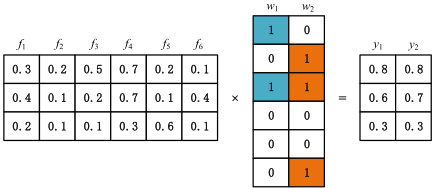
where M is a d × l row-sparse weight matrix constrained by l2,1-regularization to select common features and λ2 is the balance factor.
Furthermore, considering that the label correlation has shown its strong power in improving LDL algorithms, such as [Zheng et al., 2018; Jia et al., 2018], we prefer to exploit the label correlation at the same time. In LLSF [Huang et al., 2015], it assumes that if two labels are strongly correlated, the similarity between their coefficient vectors will be large. However, this assumption will make the corresponding specific features tend to be the same when the two labels are correlated, which is not sufficient to characterize all possible relationships between features and labels. As shown in Fig. 1, y1 is determined by the specific features {f1, f3} and y2 is determined by {f2, f3, f6}. Even if y1 and y2 are equal, their corresponding coefficient vectors w1 = [101000]T and w2 = [011001]T are different. Thus, we try to constrain label correlations directly on the output of labels, which can implicitly explore the complex relationship between features and labels.
where Rpq denotes the correlation between the p-th and the q-th labels, which is obtained by Pearson's correlation theory, and λ3 is the balance factor. Eq. 4 can be derived in the following form,
where P is the diagonal matrix with diagonal R × 1l. The first term is the loss function to measure the distance between the predicting label distribution and the ground truth. The specific features are extracted to each label according to the second term. The third term is used to capture common features that have common discrimination for all labels. And the label correlation is utilized by the last term.
3.2 Optimization
ADMM (Alternating Direction Method of Multipliers) [Boyd et al., 2011] which is suitable for addressing those objective functions with linear constraints, is proper for solving Eq. 5. To use ADMM, we first rewrite our objective into the following equivalent form,
Eq. 6 can be solved by the following alternative methods in iteration t:
Algorithm 1: The LDLSF Framework
Initialization: Q0 , W 0 , M 0 , Γ01 , Γ02 , λ01 , λ02 , λ03 , ρ, t = 1; Compute the label correlation matrix R; while stopping criterion is not satisfied do update Qt+1 by solving Eq. 7 using L-BFGS; solve W t+1 by Eq. 12; solve M t+1 by Eq. 13; update Γt+1 1 by Eq. 10; update Γt+1 2 by Eq. 11; t = t + 1; endwhere Γ1 ∈ Rd×l and Γ2 ∈ Rn×1 are the Lagrange multipliers, ρ is the penalty factor and 〈·,·〉 is the Frobenius dotproduct. For the non-negative constraint, we simply use the projection operator to set the element of XQ that does not satisfy the condition to 0.
Eq. 8 and Eq. 9 can be rewritten as follows:
Both Eq. 12 and Eq. 13 have closed form solution [Wright et al., 2009; Liu et al., 2010]. Thus, the problem remained is how to solve Eq. 7. Here, we intend to use the limitedmemory quasi-Newton method (L-BFGS) to solve it. For the optimization, the computation of L-BFGS is mainly related to the first-order gradient, which can be obtained by:
The overall procedure of the proposed LDLSF algorithm is shown in Algorithm 1.
4 Experiments
In this part, we will evaluate the proposed method on five realworld data sets with seven state-of-the-art LDL approaches over five different measures.
4.1 Data Sets
We execute our experiments on five label distribution data sets, including two facial expression data sets s-JAFFE and SBU 3DFE [Geng, 2016], and three image sentiment data sets, i.e., Emotion6 [Peng et al., 2015], Flickr LDL and Twitter LDL [Yang et al., 2017b].
| Index | Data sets | #examples | #features | #labels |
|---|---|---|---|---|
| 1 | s-JAFFE | 213 | 243 | 6 |
| 2 | SBU 3DFE | 2500 | 243 | 6 |
| 3 | Emotion6 | 1980 | 168 | 7 |
| 4 | Flickr LDL | 11150 | 168 | 8 |
| 5 | Twitter LDL | 10045 | 168 | 8 |
s-JAFFE and SBU 3DFE are extensions of two widely used facial expression image databases, i.e., JAFFE [Lyons et al., 1998] and BU 3DFE [Yin et al., 2006]. s-JAFFE contains 213 grayscale expression images with 243-dimensional features. Each image is scored by 60 persons on the six basic emotion labels (i.e., happiness, sadness, surprise, fear, anger, and disgust) with a 5-level scale. The average score of each emotion is used to represent the emotion intensity. Similarly, SBU 3DFE contains 2500 facial expression images and each image is scored by 23 persons in the same way.
Emotion6 is assembled from Flickr for a sentiment prediction benchmark, which is annotated with the votes for seven emotional categories (i.e., anger, disgust, joy, fear, sadness, surprise and neutral), containing a total of 1980 images. Flickr LDL and Twitter LDL contain 11,150 and 10,045 images respectively, whose labels fall in the typical eight-emotional space (i.e., anger, amusement, awe, contentment, disgust, excitement, fear and sadness). The features of the images in above three data sets are extracted by three popular descriptors, i.e., LBP [Ojala et al., 2002], HOG [Dalal and Triggs, 2005] and Color Moment. Since the features we extracted are high-dimensional, we use PCA to reduce the dimensionality to 168. The details of the five data sets are summarized in Table 1.
4.2 EvaluationMeasures
Five different measures [Geng, 2016] are used to evaluate the performances of the LDL algorithms. These measures can be divided into two groups: Sφrensen, Kullback-Leibler and Chebyshev are in one group to measure the distance between two vectors; the lower the values of these measures, the better the performance. Intersection and Cosine are in the other group to measure similarity, for which higher values indicate better performance.
4.3 Experimental Setting
The proposed LDLSF algorithm is compared with seven state-of-the-art algorithms: PT-Bayes, AA-kNN, SABFGS [Geng, 2016], SA-IIS [Geng et al., 2010], CPNN [Geng et al., 2013], LDL-SCL [Zheng et al., 2018] and LLSF [Huang et al., 2015]. The last five algorithms are specially designed for LDL, which can directly model the relative importance of each label to the particular instance. SA-IIS aims to minimize the Kullback-Leibler divergence between the ground truth and the predicting distribution by using improved iterative scaling method (IIS). Since IIS often performs worse than several other optimization algorithms [Malouf, 2002], an improved method SABFGS is proposed to optimize the target function through the quasi-Newton method BFGS. CPNN tries to use a three layer neural network to learn the label distribution and LDLSCL is designed based on the label correlations. LLSF is a method which learns specific features to each label for multilabel classification. This algorithm can directly deal with LDL problems by adding two LDL constraints on the model, namely LLSF-LDL. All the codes are shared by original authors, and we use the suggested parameters reported in corresponding literature, except that we tune the trade-off parameters from 10{-4,-3,··· ,2,3} for LDL-SCL and tune the parameters from 2{10,-9,··· ,9,10} for LLSF-LDL using ten-fold cross-validation. The number of cluster is set to 6 in LDLSCL.
| Measure | Algorithm | s-JAFFE | SBU 3DFE | Emotion6 | Flickr LDL | Twitter LDL |
|---|---|---|---|---|---|---|
| SA-IIS | 0.1535±0.0086 | 0.1607±0.0031 | 0.4359±0.0001 | 0.4503±0.0000 | 0.5057±0.0000 | |
| SA-BFGS | 0.1305±0.0048 | 0.1585±0.0018 | 0.4709±0.0010 | 0.3782±0.0007 | 0.3777±0.0006 | |
| AA-kNN | 0.1291±0.0056 | 0.1554±0.0024 | 0.4513±0.0013 | 0.3958±0.0005 | 0.4017±0.0007 | |
| PT-Bayes | 0.1534±0.0001 | 0.1613±0.0000 | 0.6000±0.0018 | 0.5710±0.0010 | 0.5700±0.0017 | |
| Sφrensen ↓ | CPNN | 0.1556±0.0082 | 0.1601±0.0028 | 0.5534±0.0052 | 0.4284±0.0009 | 0.4248±0.0021 |
| LLSF-LDL | 0.1450±0.0037 | 0.1573±0.0014 | 0.4203±0.0030 | 0.3834±0.0021 | 0.3744±0.0006 | |
| LDL-SCL | 0.1148±0.0086 | 0.1421±0.0035 | 0.4197±0.0040 | 0.3820±0.0022 | 0.3963±0.0032 | |
| LDLSF | 0.1126±0.0009 | 0.1353±0.0002 | 0.4237±0.0006 | 0.3753±0.0004 | 0.3680±0.0002 | |
| SA-IIS | 0.0744±0.0110 | 0.0821±0.0027 | 0.6095±0.0004 | 0.6734±0.0001 | 0.8127±0.0001 | |
| SA-BFGS | 0.0559±0.0092 | 0.0798±0.0022 | 1.1920±0.0034 | 0.7203±0.0037 | 0.6759±0.0031 | |
| AA-kNN | 0.0579±0.0080 | 0.0870±0.0045 | 0.8776±0.0134 | 10.2733±0.0073 | 1.6758±0.0072 | |
| PT-Bayes | 0.0738±0.0000 | 0.0851±0.0000 | 3.9536±0.0475 | 2.0693±0.0130 | 2.4935±0.0128 | |
| K-L ↓ | CPNN | 0.0760±0.0092 | 0.0812±0.0031 | 1.4461±0.0445 | 0.8705±0.0081 | 0.8920±0.0156 |
| LLSF-LDL | 0.0641±0.0026 | 0.0725±0.0010 | 2.9096±0.0370 | 2.3642±0.0275 | 3.0087±0.0098 | |
| LDL-SCL | 0.0443±0.0058 | 0.0627±0.0028 | 0.6084±0.0122 | 0.6230±0.0073 | 0.6600±0.0074 | |
| LDLSF | 0.0418±0.0006 0.1221±0.0103 | 0.0614±0.0003 0.1337±0.0029 | 0.6013±0.0025 0.3246±0.0001 | 0.6182±0.0020 0.3804±0.0000 | 0.6081±0.0022 0.4049±0.0000 | |
| SA-IIS SA-BFGS | 0.1040±0.0055 | 0.1325±0.0022 | 0.3721±0.0009 | 0.3006±0.0006 | ||
| AA-kNN | 0.3133±0.0005 | |||||
| 0.1034±0.0063 | 0.1305±0.0025 | 0.3340±0.0009 | 0.3322±0.0003 | 0.3217±0.0006 | ||
| PT-Bayes | 0.1204±0.0001 | 0.1389±0.0000 | 0.5240±0.0028 | 0.5045±0.0010 | 0.4970±0.0016 | |
| Chebyshev ↓ | CPNN | 0.1231±0.0098 | 0.1364±0.0029 | 0.4178±0.0057 | 0.3608±0.0011 | 0.3356±0.0015 |
| LLSF-LDL | 0.1149±0.0051 | 0.1312±0.0014 | 0.3100±0.0037 | 0.3332±0.0027 | 0.2959±0.0009 | |
| LDL-SCL | 0.0890±0.0069 | 0.1193±0.0036 | 0.3122±0.0048 | 0.3147±0.0022 | 0.3102±0.0031 | |
| LDLSF | 0.0871±0.0007 | 0.1075±0.0002 | 0.3070±0.0005 | 0.3112±0.0004 | 0.3050±0.0001 | |
| SA-IIS | 0.8465±0.0086 | 0.8393±0.0031 | 0.5641±0.0001 | 0.5497±0.0000 | 0.4943±0.0000 | |
| SA-BFGS | 0.8695±0.0048 | 0.8415±0.0018 | 0.5122±0.0010 | 0.6035±0.0007 | 0.6229±0.0006 | |
| AA-kNN | 0.8709±0.0056 | 0.8446±0.0024 | 0.5487±0.0013 | 0.6041±0.0005 | 0.5983±0.0007 | |
| PT-Bayes | 0.8466±0.0001 | 0.8387±0.0000 | 0.4000±0.0018 | 0.4316±0.0009 | 0.4337±0.0016 | |
| Intersection ↑ | CPNN | 0.8444±0.0082 | 0.8399±0.0028 | 0.4466±0.0052 | 0.5716±0.0009 | 0.5752±0.0021 |
| LLSF-LDL LDL-SCL | 0.8550±0.0037 | 0.8427±0.0014 | 0.5791±0.0030 | 0.6441±0.0019 0.6208±0.0023 | 0.6289±0.0007 | |
| 0.8851±0.0086 | 0.8579±0.0036 | 0.5763±0.0006 | 0.6247±0.0004 | 0.6320±0.0002 | ||
| LDLSF | 0.8873±0.0009 | 0.8640±0.0002 | 0.5803±0.0040 | 0.6077±0.0032 | ||
| Cosine ↑ | SA-IIS | 0.9299±0.0095 | 0.9201±0.0024 | 0.7060±0.0002 | 0.7799±0.0001 | 0.7664±0.0001 |
| SA-BFGS | 0.9470±0.0082 | 0.9221±0.0019 | 0.6158±0.0019 | 0.7547±0.0004 | 0.8140±0.0008 | |
| AA-kNN | 0.9444±0.0062 | 0.9152±0.0035 | 0.6505±0.0020 | 0.7722±0.0005 | 0.7848±0.0005 | |
| PT-Bayes CPNN | 0.9304±0.0000 0.9282±0.0083 | 0.9177±0.0000 0.9207±0.0026 | 0.5350±0.0019 0.5254±0.0069 | 0.5854±0.0012 0.7378±0.0017 | 0.5797±0.0017 0.7689±0.0025 | |
| LLSF-LDL | 0.9374±0.0034 | 0.9233±0.0010 | 0.7152±0.0037 | 0.7883±0.0023 | 0.8201±0.0012 | |
| LDL-SCL | 0.9583±0.0056 | 0.9381±0.0027 | 0.7079±0.0050 | 0.8090±0.0032 | 0.8174±0.0041 | |
| LDLSF | 0.9615±0.0006 | 0.9442±0.0001 | 0.7162±0.0010 | 0.8237±0.0001 | ||
| 0.8142±0.0002 |
| Measure | FF | critical value |
|---|---|---|
| Sφrensen | 15.0909 | 2.3593 |
| K-L | 11.3285 | |
| Chebyshev | 13.2131 | |
| Intersection | 16.0000 | |
| Cosine | 15.8113 |
In LDLSF, the parameters λ1, λ2 and λ3 are selected from 10{-6,-5,··· ,-2,-1} , respectively, and ρ is simply set as 10-3 . Besides, Q is initialized by the identity matrix. Both W and M are diagonal matrices in which all diagonal elements are 0.5. The initialization of other variables is all-zero.
4.4 Results and Discussion
Table 2 reports the detailed experimental results of eight comparing algorithms on all data sets, where the best performance among the comparing algorithms on each measure is marked in bold. On each data set, ten times ten-folds cross-validation is conducted and the mean value and standard deviation of each evaluation criterion is recorded.
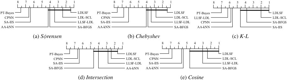
To perform comparative analysis in more well-founded ways, Friedman test is further examined which is a favorable statistical test for comparisons of more than two algorithms over multiple data sets [Demˇsar, 2006]. Table 3 summarizes the Friedman statistics FF and the corresponding critical value on each measure. As shown in Table 3, for each measure, the null hypothesis of indistinguishable performance at 0.05 significance level among the comparing algorithms is clearly rejected. Consequently, Bonferroni-Dunn test [Demˇsar, 2006] at 0.05 significance level is employed to test whether our proposed method LDLSF achieves competitive performance against the comparing algorithms, where LDLSF is considered as the control algorithm. The performance between two algorithms is significantly different if their average ranks over all data sets differ by at least one critical difference (CD). Figure 2 shows the CD diagrams on each measure. In each sub-figure, any comparing algorithm whose average rank is within one CD to that of LDLSF is connected. Otherwise, any algorithm not connected with LDLSF is considered to have significant different performance between them.
Based on these experimental results, the following observations can be made: (1) As shown in Table 2, it can be observed that the performance of proposal is better than other algorithms in general. (2) As shown in Fig. 2, LDLSF achieves optimal average rank in terms of all evaluation metrics. In detail, LDLSF significantly outperforms PT-Bayes and CPNN on all the measures. Moreover, the proposal significantly outperforms SA-IIS on all metrics except for K-L and outperforms AA-kNN in terms of K-L and Cosine. Besides, LDLSF is comparable to LDL-SCL and SA-BFGS based on all evaluation metrics, comparable to LLSF-LDL in terms of Sφrensen, Chebyshev, Intersection and Cosine.
In summary, the proposed LDLSF algorithm achieves a competitive performance against other well-established label distribution algorithms. The results demonstrate the effectiveness of LDLSF.
4.5 Convergence
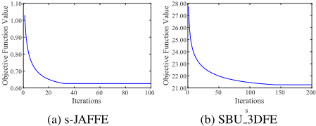
To investigate the convergence of the ADMM algorithm in solving LDLSF model, we plot the values of the objective function on two data sets (s-JAFFE and SBU 3DFE) in Figure 3. As can be observed, the value decreases as the number of iterations increases. In detail, the objective function on sJAFFE approaches a fixed value at about 32 iterations, while it reaches a fixed value on SBU 3DFE after approximately 150 iterations.
5 Conclusions
In this paper, we proposed a novel LDL algorithm by jointing label-specific feature learning, common feature learning and label correlations simultaneously. The label-specific features are extracted by exploiting the l1-regularization and the common features which may be ignored by l1-regularization are learned by utilizing the l2,1-regularization. Then, the label correlations are concerned by directly modeling the output of labels. The experimental results on several real-world data sets demonstrate the effectiveness of LDLSF.
Acknowledgements
This work is jointly supported by the National Key R&D Program of China (No. 2018YFB1003902), Natural Science Foundation of Jiangsu Province (Nos. BK20170809, BK20170033), the National Natural Science Foundation of China (Nos. 61773208, 61872190, 61772275, 71671086), and Jiangsu Key Laboratory of Big Data Security and Intelligent Processing (NJUPT).
@inproceedings{ijcai2019p460,
  title     = {Label distribution learning with label-specific features},
  author    = {Ren, Tingting and Jia, Xiuyi and Li, Weiwei and Chen, Lei and Li, Zechao},
  booktitle = {Proceedings of the Twenty-Eighth International Joint Conference on
               Artificial Intelligence, {IJCAI-19}},
  publisher = {International Joint Conferences on Artificial Intelligence Organization},
  editor    = {Sarit Kraus},
  pages     = {3318--3324},
  year      = {2019},
  month     = {8},
  note      = {Main track},
  doi       = {10.24963/ijcai.2019/460},
  url       = {https://doi.org/10.24963/ijcai.2019/460},
}
TY - CPAPER TI - Label distribution learning with label-specific features AU - Ren, Tingting AU - Jia, Xiuyi AU - Li, Weiwei AU - Chen, Lei AU - Li, Zechao T2 - Proceedings of the Twenty-Eighth International Joint Conference on Artificial Intelligence, IJCAI-19 PB - International Joint Conferences on Artificial Intelligence Organization PY - 2019 SP - 3318 EP - 3324 DO - 10.24963/ijcai.2019/460 UR - https://doi.org/10.24963/ijcai.2019/460 ER -Copied
Machine-readable versions of this paper, for tools and AI agents:





