
Rapid Performance Gain through Active Model Reuse
Proceedings of the Twenty-Eighth International Joint Conference on Artificial Intelligence. Main track. Pages 3404-3410.
https://doi.org/10.24963/ijcai.2019/472
Keywords
- Machine Learning: Active Learning
- Machine Learning: Classification
Abstract
Model reuse aims at reducing the need of learning resources for a newly target task. In previous model reuse studies, the target task usually receives labeled data passively, which results in a slow performance improvement. However, learning models for target tasks are often required to achieve good enough performance rapidly for practical usage. In this paper, we propose the AcMR (Active Model Reuse) method for the rapid performance improvement problem. Firstly, we construct queries through pre-trained models to facilitate the active learner when labeled examples are insufficient in the target task. Secondly, we consider that pre-trained models are able to filter out not-very-necessary queries so that AcMR can save considerable queries compared with direct active learning. Theoretical analysis verifies that AcMR requires fewer queries than direct active learning. Experimental results validate the effectiveness of AcMR.
- [Albrecht, 2016] Jan Philipp Albrecht. How the gdpr will change the world. European Data Protection Law Review, 2:287, 2016.
- [Chakraborty et al., 2015] Shayok Chakraborty, Vineeth Balasubramanian, Qian Sun, Sethuraman Panchanathan, and Jie-Ping Ye. Active batch selection via convex relaxations with guaranteed solution bounds. IEEE Trans- actions on Pattern Analysis and Machine Intelligence, 37(10):1945-1958, 2015.
- [Dietterich, 2000] Thomas G Dietterich. Ensemble methods in machine learning. In International Workshop on Mul- tiple Classifier Systems, pages 1-15, Günzburg, Germany, 2000.
- [Harrell, 2015] Frank E Harrell. Ordinal logistic regression. In Regression modeling strategies, pages 311-325. 2015.
- [He et al., 2018] Kai-Ming He, Ross Girshick, and Piotr Dollár. Rethinking imagenet pre-training. arXiv preprint arXiv:1811.08883, 2018.
- [Huang et al., 2010] Sheng-Jun Huang, Rong Jin, and Zhi- Hua Zhou. Active learning by querying informative and representative examples. In Advances in Neural Infor- mation Processing Systems, pages 892-900, Vancouver, Canada, 2010.
- [Kingma and Ba, 2014] Diederik P Kingma and Jimmy Ba. Adam: A method for stochastic optimization. arXiv preprint arXiv:1412.6980, 2014.
- [Lewis and Gale, 1994] David D Lewis and William A Gale. A sequential algorithm for training text classifiers. In Pro- ceedings of the 17th International ACM SIGIR Conference on Research and Development in Information Retrieval, pages 3-12, 1994.
- [Li and Liang, 2019] Yu-Feng Li and De-Ming Liang. Safe semi-supervised learning: a brief introduction. Frontiers of Computer Science, pages 1-8, 2019.
- [Li et al., 2013] Nan Li, Ivor W Tsang, and Zhi-Hua Zhou. Efficient optimization of performance measures by classi- fier adaptation. IEEE transactions on Pattern Analysis and Machine Intelligence, 35(6):1370-1382, 2013.
- [Li et al., 2017] Yu-Feng Li, Han-Wen Zha, and Zhi-Hua Zhou. Learning safe prediction for semi-supervised re- gression. In Proceedings of the 31st AAAI Conference on Artificial Intelligence, volume 2017, pages 2217-2223, San Francisco, CA, 2017.
- [Li et al., 2019] Yu-Feng Li, Hai Wang, Tong Wei, and Wei- Wei Tu. Towards automated semi-supervised learning. In Proceedings of the 33rd AAAI conference on Artificial In- telligence, Honolulu, HI, 2019.
- [Long et al., 2017] Ming-Sheng Long, Han Zhu, Jian-Min Wang, and Michael I Jordan. Deep transfer learning with joint adaptation networks. In Proceedings of the 34th International Conference on Machine Learning, pages 2208-2217, Sydney, Australia, 2017.
- [Murugesan et al., 2016] Keerthiram Murugesan, Han-Xiao Liu, Jaime Carbonell, and Yi-Ming Yang. Adaptive smoothed online multi-task learning. In Advances in Neu- ral Information Processing Systems, pages 4296-4304, Barcelona, Spain, 2016.
- [Pan and Yang, 2010] Sinno Jialin Pan and Qiang Yang. A survey on transfer learning. IEEE Transactions on Knowl- edge and Data Engineering, 22(10):1345-1359, 2010.
- [Pan et al., 2011] Sinno Jialin Pan, Ivor W Tsang, James T Kwok, and Qiang Yang. Domain adaptation via transfer component analysis. IEEE Transactions on Neural Net- works, 22(2):199-210, 2011.
- [Parkhi et al., 2015] Omkar M. Parkhi, Andrea Vedaldi, and Andrew Zisserman. Deep face recognition. In Proceedings of the 26th British Machine Vision Conference, Swansea, UK, 2015.
- [Settles, 2012] Burr Settles. Active learning. Synthesis Lectures on Artificial Intelligence and Machine Learning, 6(1):1-114, 2012.
- [Seung et al., 1992] H Sebastian Seung, Opper Manfred, and Sompolinsky Haim. Query by committee. In Proceedings of the 5th Annual Workshop on Computational Learning Theory, pages 287-294, Pittsburgh, PA, 1992.
- [Shi et al., 2008] Xiao-Xiao Shi, Wei Fan, and Jiang-Tao Ren. Actively transfer domain knowledge. In Proceed- ings of Joint European Conference on Machine Learning and Knowledge Discovery in Databases, pages 342-357, Antwerp, Belgium, 2008.
- [Wang and Ye, 2015] Zheng Wang and Jie-Ping Ye. Query- ing discriminative and representative samples for batch mode active learning. ACM Transactions on Knowledge Discovery from Data, 9(3):17, 2015.
- [Yang et al., 2017a] Yang Yang, De-Chuan Zhan, Ying Fan, Yuan Jiang, and Zhi-Hua Zhou. Deep learning for fixed model reuse. In Proceedings of the 31st AAAI Conference on Artificial Intelligence, pages 2831-2837, San Fran- cisco, CA, 2017.
- [Yang et al., 2017b] Yang Yang, De-Chuan Zhan, Xiang-Yu Guo, and Yuan Jiang. Modal consistency based pre-trained multi-model reuse. 2017. IJCAI
- [Ye et al., 2018] Han-Jia Ye, De-Chuan Zhan, Yuan Jiang, and Zhi-Hua Zhou. Rectify heterogeneous models with semantic mapping. In Proceedings of the 35th Inter- national Conference on Machine Learning, pages 1904- 1913, Stockholm, Sweden, 2018.
- [Zhou, 2012] Zhi-Hua Zhou. Ensemble Methods: founda- tions and algorithms. 2012.
- [Zhou, 2016] Zhi-Hua Zhou. Learnware: on the future of machine learning. Frontiers of Computer Science, 10(4):589-590, 2016.
References were extracted automatically from the PDF and may contain errors.
Full text extracted automatically from the PDF; figures, tables and equations may differ. The PDF is the version of record.
1 Introduction
In traditional machine learning, a learning model is tailored to the target task. Nowadays, however, with the popularity of machine learning, unlike training data which is often hard to share due to the privacy issue [Albrecht, 2016], a great deal of well-trained machine learning models have been available for use. For example, these models have been trained with a large amount of labeled training data [Parkhi et al., 2015]; with smart optimization techniques [Kingma and Ba, 2014]. All these models work well on the specific tasks, but have to be discarded once the target task changes, which causes the user to retrain a newmodel for the target task.
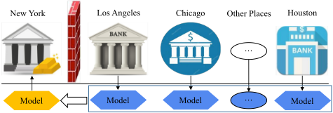
Model reuse [Zhou, 2016] tries to reduce the learning resources for a new target task with the exploitation of pretrained models (as demonstrated in Figure 1), which has attracted much attention and has shown promising performance when the labeled examples are limited for the target task. For example, Yang et al. [2017b] makes predictions for new instances from a collection of different pre-trained models and shows encouraging results; Ye et al. [2018] adapts the pretrained models to a new environment with different features and shows that the performance will be boosted. However, previous model reuse studies usually assume that the labeled data for the target task are passively collected. This leads to a limited performance improvement for the target task, which may be difficult to meet the demands. Since in many practical applications, it is expected that the performance of the target model can be good enough and quickly improved. It is evident that this scenario is quite different from the classic model reuse studies. We call this kind of model reuse the "rapid performance improvement" problem.
The problem is related to but different to standard active learning [Settles, 2012], which tries to select the most informative instances to be labeled. The informativeness is typically defined as maximal expected improvement in classification accuracy [Huang et al., 2010]. Many sample selection criteria (e.g., uncertainty sampling [Lewis and Gale, 1994], query by committee (QBC) [Seung et al., 1992]) have been devoted. However, they ignore the use of many pre-trained models, which results in a slow performance improvement for target tasks or needing a large amount of query costs.
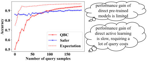
As illustrated in Figure 2, for a new classification task in 20 Newsgroups, we directly employ active learning method (e.g., QBC [Seung et al., 1992]) or model reuse method (e.g., Safer [Li et al., 2017]). As shown, both of the two approaches yield slow performance gains or require a large number of queries to achieve good enough accuracy.
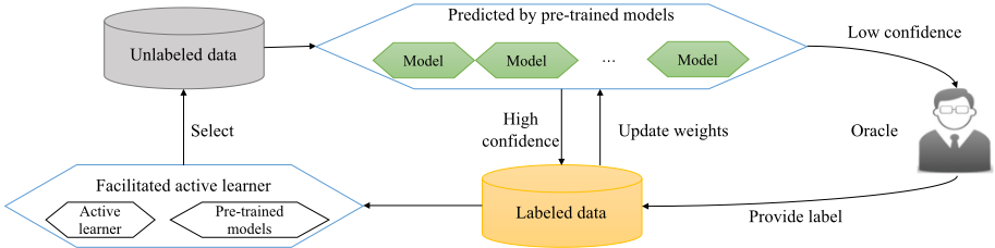
In this paper, we study the rapid performance improvement problem and propose the ACMR (Active Model Reuse) method. As illustrated in Figure 3, unlike traditional active learning, we consider pre-trained models to help construct queries, facilitating active learner when labeled examples are insufficient on the target task. Moreover, we leverage pretrained models to filter out not very necessary queries so that considerable queries could be saved compared with direct active learning. During the learning process, the relationships between pre-trained models and the target task are continually updated such that they can predict unlabeled samples more accurately. Theoretical analysis verifies that ACMR requires fewer queries than active learning. Experiments show the superior performance of the proposed method.
This paper is structured as follows. We first review related works and then present our proposed method. Next we show the experiments. Finally we conclude this work.
2 RelatedWork
Reusability has been emphasized as a crucial characteristic of the new concept of learnware [Zhou, 2016]. It would be ideal if models can be reused in scenarios that are very different from their original training ones. This is of course a big challenge, whereas reusing models have already been demonstrated very useful. Li et al. [2013] has shown that by starting from a trained model, it is easier to construct a model. FMR [Yang et al., 2017a] integrates the discriminative ability of fixed models into deep network training, and achieves promising performance in various applications.
Active learning tries to query the most informative samples and mainly focuses on representative and uncertain information in the unlabeled data [Settles, 2012]. For example, one of the most common strategies is the uncertainty-based selection [Lewis and Gale, 1994], in which the certainties are measured according to the predictions on new unlabeled samples obtained from the initial classifiers. Chakraborty et al. [2015] combines the uncertainty and representativeness into a convex framework to perform active learning loops. Huang et al. [2010] queries the informative and representative samples based on a min-max framework. Wang and Ye [2015] puts the discrimination and representativeness together via a trade-off parameter to query the i.i.d samples.
Transfer learning is one way of implementing model reuse. However, it typically works on a more general problem setting [Pan and Yang, 2010], such as transferring knowledge through data representation [Pan et al., 2011], model structures [Long et al., 2017] and so on. There are several studies on actively transfer learning [Shi et al., 2008], however, they require additional data rather than strict model reuse setting.
| Notation | Meaning |
|---|---|
| N yt ∈ {+1, -1} L U {f1, f2, . . . , fk} f (t) j η = [η1, η2, . . . , ηk] l(t) j = (1 - y(t) f (t) j )+ Lj = ∑xt∈L l(t) j fL f (t) L | number of training data ture label of instance xt labeled data in the target task unlabeled data in the target task k pre-trained models the prediction of fj on xt the weight vector of k models the hinge loss of j-th model for xt the empirical loss of j-th model the active learner built on L the prediction of fL on xt |
In recent years, robust model reuse based on semisupervised learning [Li et al., 2017; Li and Liang, 2019; Li et al., 2019] has been proposed, which works on deriving performance-safe prediction when labeled examples in target tasks are limited, where safe prediction means that the performance would not be worse than direct supervised learning using only limited labeled data. Although these studies are able to achieve prudent performance, the performance improvement is often relatively limited since they never consider involving more labeled data.
3 The ACMRMethod
3.1 Notation and Setting
Let D = {(x1, y1), (x2, y2), . . . , (xnl , ynl ), xnl+1, . . . , xN} be the training data set of the target task that consists of nl labeled instances and nu = N - nl unlabeled ones. Each instance xt = [xt1, xt2, . . . , xtd]⊤ is a vector of d dimensions. L = {(x1, y1), (x2, y2), . . . , (xnl , ynl )} is the labeled data set and U = {xnl+1, . . . , xN} is the unlabeled one. Table 1 summarizes the notations in the paper.
Formally, suppose that we have obtained k pre-trained models {f1, f2, . . . , fk}. We let fL denote the active learner obtained by training a supervised learner with only labeled data. The goal of model reuse is to derive a better model: f + = g({f1, f2, . . . , fk}, fL), which often outperforms, meanwhile would not be worse than fL. g represents the form of model reuse, specifically, with the help of pre-trained models, f + can be build by structural risk minimization:
where LX = {x1, x2, . . . , xnl }, LY = {y1, y2, . . . , ynl }, L is a loss function, e.g., mean square loss, hinge loss, etc and Ω is a regularizer. The smaller the value of the loss function, the better the performance. The forms of the loss function, regularizer and f + are flexible to design for specific tasks. In this paper, we use the hinge loss and logistic regression [Harrell, 2015] to be the form of loss function and f + respectively.
3.2 Deficiencies of Baseline Approaches
Previous works on model reuse typically assume that when labeled examples for the target task are limited, model reuse could guarantee performance improvement [Ye et al., 2018; He et al., 2018]. However, this facilitation is only effective when the number of labeled samples is small and the performance improvement is often relatively limited. To get a good enough model, we still need a lot of queries.
Assume we have obtained confident weights (denoted by η = [η1, . . . , ηk]) of the pre-trained models about the target task, according to the weighted voting method [Dietterich, 2000], the prediction ˆ y(t) of the unlabeled instance xt is
where I(z) = 1 if z is true and 0 otherwise. This prediction, however, may be risky since we can not get accurate prior weights especially when there are very few labeled examples in target tasks [Pan and Yang, 2010]. As illustrated in Figure 2, we consider that the pre-trained models are helpful while their performance is not good enough.
Thus, rather than fully trusting pre-trained models, we consider trusting the pre-trained models partially and leverage pre-trained models to filter out not very necessary queries generated by direct active learning to facilitate an effective active learner. Moreover, once the label capacity is enhanced, we continually update the confident weights of pre-trained models to improve their confidence for target task. It is worthy that the above two steps promote each other in the active learning iterations. In the following, we introduce them respectively and present the theoretical justification.
3.3 Actively Reuse Pre-trainedModels
When the predictions of pre-trained model are risky, we may have the following observations [Shi et al., 2008]: i) Pretrained models assign xt with a class label that is different from the one given by the facilitated active learner; ii) The posteriors of the pre-trained models are low.
According to the above considerations, we can design a query indicator function θ(xt) to reflect the necessity for unlabeled instance xt to query the label:
Pj (ˆ y(t) |xt) is the predicted probability of pre-trained model fj for instance xt. As it can be seen, α(xt) is related to the posteriori probability P(ˆ y(t) |xt), and α(xt) = 0 if the supervised classifier f (t) L and the pre-trained models have assigned different labels to xt. In general, the larger the value α(xt) is, the less we need to query the label.
Moreover, because mislabeling of the few instances can put significant negative effect on accuracy, we further set θ(xt) = (1+α(xt))-1 so as to guarantee the possibility (necessity) to query is greater than 50%. In other words, we trust the label given by the pre-trained models only when its confidence reflected by α(xt) is very high. Accordingly, with the value of θ(xt), we randomly generate a real number R within 0 to 1, and then the decision function F(xt) is defined as
According to Eq.(6), if F(xt) = 0, then it means that the instance xt should be labeled by the pre-trained models; otherwise, xt should be labeled by the domain experts. In other words, we label the instance xt by the pre-trained models with probability 1 - θ(xt).
We then derive its sampling error bound to demonstrate its ability to mitigate the deficiencies for direct approaches, which utilizes the predictions only when they are accurate enough. Additionally, we show its querying bound to validate the claim that ACMR can reduce labeling cost by querying fewer examples. In the algorithm ACMR, let εp and εa denote the expected error of the pre-trained models and the active learner fL respectively, and let δ = εp + εa. The results of theoretical analysis are shown in Table 2.
Theorem 1. In the algorithm ACMR, we assume that εa ≤ εp, then the sampling error ε for ACMR satisfies:
| Evaluation Criterion | Bound of Value |
| Sampling Error | ε2p 1+(1-εp) |
| Querying Rate | δ + 1-δ 1+(1-εp) |
Proof. According to the analysis of the decision function F(x) described above, ACMR makes wrong decision only when both the pre-trained models and the active learner fL agree on the wrong label. In this case, ACMR has probability 1 - θ(x) to trust the classification result given by the pre-trained models, where θ(x) is defined in Eq.(5). Thus, the sampling error of ACMR can be written as ε = εpεa(1 - θ(x)) ≤ ε2p (1 - θ(x)). Moreover, in this situation, θ(x) = 1 1+(1-εp) . Thus,
Theorem 2. In the algorithm ACMR, for an unlabeled instance, the probability that ACMR queries the label from the experts (with cost) satisfies:
Proof. According to the analysis of the decision function F(x), ACMR will query the experts to label the instance when the pre-trained models and the active learner hold different predictions on the classification result. And when the two classifiers agree on the result, it still has probability θ(x) to query the experts. Thus:
Remark. In contrast to Shi et al. [2008] which suffers from exponential term exp(-N -1 ), the results in Theorem 1 and Theorem 2 show that ACMR avoid this issue and improve the bound evidently. From theoretical analysis, we can find that the sampling error and querying probability of the proposed approach are bounded and related to εp and εa. In the next section we will talk about how to reduce εp to improve performance in the whole learning process.
3.4 UpdateWeights for Pre-TrainedModels
It is well known that ensemble learning often outperforms individual models [Zhou, 2012]. However, simply building a uniformly weighted ensemble of the models is suboptimal, since it does not measure the precise relationships between each pre-trained model and the target task.
Inspired by Murugesan et al. [2016], we employ an errordriven update rule in which the weights of pre-trained models
Algorithm 1 The learning algorithm for ACMR
Input: labeled dataset L, unlabeled dataset U, sampling size N, k pre-trained models {f1, f2, . . . , fk} and λ > 0 Output: the model fL for the target task
- 1: Initialize weight vector η = [1/k, ..., 1/k] and fL.
- 2: for m= 1, 2, · · · ,N do
- 3: Select an instance xt(m) from U by traditional active learning
- 4: Predict xt(m) by pre-trained models, and calculate the decision function F(xt(m)) via Eq.(6)
- 5: if F(xt(m)) = 0 then
- 6: yt(m) ← ˆ y(t(m))
- 7: else
- 8: yt(m) ← query from oracle
- 9: if yt(m) ̸= ˆ y(t(m)) then
10:
update the weights via Eq.(12)
- 11: else
- 12: η(m+1) ← η(m)
- 13: end if
- 14: end if
- 15: L = L∪ (xt(m), yt(m)), U = U/(xt(m));
- 16: Train the learner fL with L
- 17: Facilitate active learner fL via Eq.(1)
- 18: end for
- 19: return fL
are updated only when the prediction of pre-trained models is wrong. Specifically, at time m, the target task receives a training instance xt(m), the pre-trained models make a prediction and suffer a loss after yt(m) is revealed. Following the error-driven update rule in which the weights are updated only when the pre-trained models make a mistake, we consider the following optimization problem at each time:
where DKL(η||η(m) ) denotes the Kullback-Leibler (KL) divergence between current and previous soft-attention distributions, which allows η to evolve smoothly over time. The solution for η(m+1) is given in a closed form:
Proposition 1. (Weight Concentration). During the weight update procedure in the whole learning process, the weights will concentrate on those pre-trained models who suffer a small cumulative loss on the target task.
Proof. Through the update rule, we know that the weight associated with the j-th previous model is equal to ηj = exp(-Lj /λ) ∑kj′=1 exp(-Lj′/λ) , j ∈ [k]. The smaller the loss Lj of the pre-trained model, the higher the weight ηj.
We summarize the pseudo-code of ACMR in Algorithm 1.
| Task | Q | Safer | QBC | AcTrak-QBC | AcMR-QBC | Random | AcTrak-Ran | AcMR-Ran |
|---|---|---|---|---|---|---|---|---|
| Task1 | 30 60 90 | .876± .033 .792± .880± .029 .916± .891± .040 .930± | .118 .029 .022 | .817± .107 .909± .052 .929± .026 | .923± .016 .932± .013 .934± .011 | .806± .126 .911± .030 .928± .025 | .839± .079 .915± .034 .934± .019 | .926± .014 .933± .008 .936± .011 |
| Task2 | 30 60 90 | .737± .027 .738± .036 .749± .038 | .739± .124 .821± .076 .856± .065 | .711± .143 .809± .091 .851± .050 | .838± .039 .870± .044 .885± .032 | .689± .110 .833± .059 .871± .032 | .756± .102 .842± .071 .861± .056 | .839± .049 .873± .038 .892± .027 |
| Task3 | 30 60 90 | .944± .010 .945± .011 .945± .010 | .788± .155 .903± .080 .937± .040 | .803± .128 .920± .049 .948± .015 | .954± .012 .956± .011 .957± .012 | .748± .146 .868± .115 .928± .043 | .839± .095 .921± .050 .951± .020 | .952± .012 .956± .011 .957± .009 |
| Task4 | 30 60 90 | .689± .059 .680± .049 .703± .040 | .705± .119 .853± .085 .907± .044 | .664± .133 .797± .126 .859± .086 | .905± .027 .928± .012 .938± .011 | .786± .142 .875± .063 .914± .032 | .757± .131 .875± .083 .922± .023 | .910± .027 .927± .018 .933± .017 |
| Task5 | 30 60 90 | .850± .061 .869± .053 .871± .057 | .765± .133 .888± .081 .925± .030 | .753± .142 .880± .065 .915± .055 | .915± .059 .941± .029 .949± .015 .819± .029 | .765± .134 .864± .085 .909± .042 .643± .104 .743± .103 | .758± .177 .833± .128 .886± .087 | .941± .015 .937± .027 .950± .011 |
| Task6 | 30 60 90 | .770± .042 .763± .042 .788± .034 | .645± .105 .679± .089 .747± .106 | .646± .093 .718± .094 .781± .081 | .838± .032 .860± .031 | .841± .083 | .676± .113 .779± .090 .823± .075 | .821± .040 .850± .038 .867± .031 |
4 Experiment
In this section, we first give the experimental setup and then show the evaluation of our proposal compared to several state-of-the-art algorithms on a number of real-world tasks.
4.1 Experimental Setup
In order to better validate our method, the following methods are compared in our experiments. Two sample selection criteria: i) QBC [Seung et al., 1992] selects examples that cause maximum disagreement amongst an ensemble of hypotheses; ii) Random selects examples randomly; one actively transfer learning method AcTraK [Shi et al., 2008]; one baseline method Safer [Li et al., 2017].
For ACMR, we choose QBC and Random to implement the base sampling strategy respectively, and we take the pretrained models as the input to ACMR. For example, in the sentiment analysis task of book, we take the pre-trained models in DVD as the input to ACMR; in the classification task of rec.autos and sci.crypt, we take the pre-trained models in "rec.motorcycles and sci.electronics" as the input to ACMR.
Because ACMR need experts to annotate unlabeled samples, we should compare these methods in different number of samples labeled by experts. For each task, we randomly divide the data into two parts: 75% as the unlabeled pool, and the rest 25% as the test set. Experiments are repeated for 30 times, and the average classification accuracy is reported.
4.2 Text Classification Task
The text classification task is collected from 20 Newsgroups 1 . 20 Newsgroups has a two-level hierarchy, for example, the four sub-categories (sci.crypt, sci.electronics, sci.med, sci.space) belong to the top-category sci. Because the difference among top-categories is relatively large and the subcategories under each top-category are similar, we can design the top-categories classification problem. For example, we generate 6 text classification tasks (comp vs. talk, comp vs. sci, comp vs. rec, rec vs. talk, rec vs. sci, sci vs. talk).
1 https://www.cse.ust.hk/TL/
Results are shown in Table 3, which can be seen that ACMR can achieve better performance than other methods. It can be seen that ACMR obtains quite promising performance as the number of queries increases, for various sample selection criteria. Actively transfer learning methods also obtain good performance but is not that competitive as ACMR. This suggests that the use of pre-trained models is beneficial to improve performance rapidly.
4.3 Sentiment Analysis Task
The second task is a sentiment analysis problem 1 , and the goal is to label the documents with respect to what types of problems they describe. We evaluate our algorithm on product reviews from Amazon on a dataset containing reviews from 4 domains: Book, DVD, Electronics and Kitchen. We consider each domain as a binary classification task: reviews with rating > 3 are labeled positive(+), those with rating < 3 are labeled negative(-). For sentiment analysis dataset we have 4 classification tasks.
Results are shown in Table 4, which can be seen that ACMR can significantly outperform its based active learning methods in most cases. Moreover, ACMR also consistently performs better as the number of labeled examples increases. More importantly, we find that even though the performance improvement of pre-trained models is very limited, our proposal can also use them to improve performance rapidly. It also clearly shows the advantage of our proposed approach which is able to exploit useful pre-trained models.
| Task | Q | Safer | QBC | AcTrak-QBC | AcMR-QBC | Random | AcTrak-Ran | AcMR-Ran |
|---|---|---|---|---|---|---|---|---|
| Task1 | 30 60 90 | .612± .022 .529± .033 .614± .018 .579± .048 .614± .018 .615± .047 | .578± .609± .627± | .033 .035 .038 | .607± .028 .631± .023 .645± .023 | .577± .036 .607± .025 .625± .024 | .582± .039 .615± .037 .637± .034 | .598± .032 .631± .026 .649± .020 |
| Task2 | 30 60 90 | .648± .020 .648± .018 .648± .020 | .562± .048 .591± .049 .621± .047 | .582± .041 .626± .038 .649± .033 | .610± .033 .631± .030 .660± .031 | .594± .031 .623± .033 .650± .026 | .594± .036 .629± .034 .657± .028 | .611± .046 .643± .032 .668± .029 |
| Task3 | 30 60 90 | .651± .044 .654± .041 .665± .033 | .578± .057 .640± .046 .672± .035 | .629± .033 .665± .024 .685± .023 | .645± .036 .676± .028 .694± .025 | .612± .036 .643± .032 .671± .027 | .629± .033 .664± .032 .679± .029 | .642± .037 .676± .026 .690± .025 |
| Task4 | 30 60 90 | .621± .049 .631± .051 .643± .054 | .628± .032 .657± .035 .684± .026 | .634± .033 .666± .024 .687± .026 | .644± .026 .680± .018 .702± .022 | .624± .036 .652± .032 .678± .026 | .628± .045 .663± .035 .681± .033 | .641± .035 .684± .029 .705± .024 |
| Task | Q | Safer | QBC | AcTrak-QBC | AcMR-QBC | Random | AcTrak-Ran | AcMR-Ran |
|---|---|---|---|---|---|---|---|---|
| Task1 | 30 60 90 | .925± .028 .757± .152 .935± .028 .778± .142 .939± .021 .788± .117 | .734± .144 .750± .116 .761± .092 | .956± .016 .954± .021 .954± .024 | .673± .148 .731± .139 .805± .143 | .681± .149 .755± .113 .806± .088 | .951± .017 .957± .018 .957± .023 | |
| Task2 | 30 60 90 | .906± .037 .908± .037 .901± .038 | .750± .163 .824± .118 .872± .097 | .770± .161 .791± .151 .838± .144 | .952± .032 .965± .017 .968± .014 | .707± .170 .787± .136 .843± .099 | .751± .159 .849± .110 .910± .078 | .949± .024 .962± .021 .960± .019 |
| Task3 | 30 60 90 | .897± .051 .914± .052 .913± .042 | .846± .116 .895± .052 .928± .039 | .875± .098 .916± .037 .908± .042 | .970± .024 .984± .014 .986± .013 | .860± .064 .895± .055 .902± .046 | .879± .047 .895± .044 .888± .039 | .965± .031 .981± .015 .983± .014 |
| Task4 | 30 60 90 | .962± .023 .964± .023 .964± .023 | .928± .072 .964± .023 .964± .023 | .924± .081 .968± .019 .968± .019 | .959± .023 .970± .019 .970± .019 | .944± .030 .959± .020 .963± .021 | .942± .022 .967± .015 .969± .012 | .961± .021 .967± .016 .973± .013 |
4.4 SpamDetection Task
The last task is a spam detection problem, and we use the dataset obtained from ECML PAKDD Discovery challenge 2 to verify whether our method can help improve the performance. We use the task B challenge dataset which consists of labeled training data from the inboxes of 15 users. Each task is a binary classification problem: spam or non-spam. For spam detection task, we test the top 4 classification tasks.
Results from Table 5 show that ACMR achieves highly competitive performance with compared methods. Once again, our proposal works better than state-of-the-art active learning and Safer model prediction algorithms. This shows that in the frame of active learning, taking pre-trained models into account can get a rapid performance improvement.
2 http://ecmlpkdd2006.org/challenge.html
5 Conclusion
Reusable model design becomes a desire for the rapid expansion of machine learning applications. However, previous model reuse studies assume that the target task receives labeled data passively. This leads to a slow performance improvement to the target task. In this paper, we study a kind of new model reuse problem, where the goal is that the model performance for the target task can be quickly improved. We propose the ACMR method which constructs queries through pre-trained models when labeled examples are insufficient for the target task, and leverages pre-trained models to filter out not very necessary queries. Extending our work into deep learning problem and applying it to more applications are interesting for future study.
Acknowledgments
This research was supported by the National Key R&D Program of China (2018YFB1004300), the National Natural Science Foundation of China (61772262) and the Fundamental Research Funds for the Central Universities (020214380053).
@inproceedings{ijcai2019p472,
  title     = {Rapid Performance Gain through Active Model Reuse},
  author    = {Shi, Feng and Li, Yu-Feng},
  booktitle = {Proceedings of the Twenty-Eighth International Joint Conference on
               Artificial Intelligence, {IJCAI-19}},
  publisher = {International Joint Conferences on Artificial Intelligence Organization},
  editor    = {Sarit Kraus},
  pages     = {3404--3410},
  year      = {2019},
  month     = {8},
  note      = {Main track},
  doi       = {10.24963/ijcai.2019/472},
  url       = {https://doi.org/10.24963/ijcai.2019/472},
}
TY - CPAPER TI - Rapid Performance Gain through Active Model Reuse AU - Shi, Feng AU - Li, Yu-Feng T2 - Proceedings of the Twenty-Eighth International Joint Conference on Artificial Intelligence, IJCAI-19 PB - International Joint Conferences on Artificial Intelligence Organization PY - 2019 SP - 3404 EP - 3410 DO - 10.24963/ijcai.2019/472 UR - https://doi.org/10.24963/ijcai.2019/472 ER -Copied
Machine-readable versions of this paper, for tools and AI agents:





