
AugBoost: Gradient Boosting Enhanced with Step-Wise Feature Augmentation
Proceedings of the Twenty-Eighth International Joint Conference on Artificial Intelligence. Main track. Pages 3555-3561.
https://doi.org/10.24963/ijcai.2019/493
Keywords
- Machine Learning: Dimensionality Reduction and Manifold Learning
- Machine Learning: Ensemble Methods
- Machine Learning: Classification
- Machine Learning: Deep Learning
Abstract
Gradient Boosted Decision Trees (GBDT) is a widely used machine learning algorithm, which obtains state-of-the-art results on many machine learning tasks. In this paper we introduce a method for obtaining better results, by augmenting the features in the dataset between the iterations of GBDT. We explore a number of augmentation methods: training an Artificial Neural Network (ANN) and extracting features from it's last hidden layer (supervised), and rotating the feature-space using unsupervised methods such as PCA or Random Projection (RP). These variations on GBDT were tested on 20 classification tasks, on which all of them outperformed GBDT and previous related work.
- [Alcala-Fdez et al., 2011] Jesus Alcala-Fdez, Alberto Fer- nandez, Julian Luengo, Joaquin Derrac, and Salvador Gar- cia. Keel data-mining software tool: Data set repository, integration of algorithms and experimental analysis frame- work. Multiple-Valued Logic and Soft Computing, 17(2- 3):255-287, 2011.
- [Breiman, 2001] Leo Breiman. Random forests. Machine learning, 45(1):5-32, 2001.
- [Burges, 2010] Christopher JC Burges. From ranknet to lambdarank to lambdamart: An overview. Learning, 11(23-581):81, 2010.
- [Casale et al., 2011] Pierluigi Casale, Oriol Pujol, and Petia Radeva. Embedding random projections in regularized gradient boosting machines. In Ensembles in Machine Learning Applications, pages 201-216. Springer, 2011.
- [Chen and Guestrin, 2016] Tianqi Chen and Carlos Guestrin. Xgboost: A scalable tree boosting system. In Proceedings of the 22nd acm sigkdd international conference on knowl- edge discovery and data mining, pages 785-794. ACM, 2016.
- [Chen et al., 2018] Hugh Chen, Scott Lundberg, and Su- In Lee. Hybrid gradient boosting trees and neuralnet- works for forecasting operating room data. arXiv preprint arXiv:1801.07384, 2018.
- [Demšar, 2006] Janez Demšar. Statistical comparisons of classifiers over multiple data sets. Journal of Machine learning research, 7(Jan):1-30, 2006.
- [Dheeru and Karra Taniskidou, 2017] Dua Dheeru and Efi Karra Taniskidou. UCI machine learning repository, 2017.
- [Freund and Schapire, 1997] Yoav Freund and Robert E Schapire. A decision-theoretic generalization of on-line learning and an application to boosting. Journal of com- puter and system sciences, 55(1):119-139, 1997.
- [Friedman, 2001] Jerome H Friedman. Greedy function ap- proximation: a gradient boosting machine. Annals of statistics, pages 1189-1232, 2001.
- [Joly, 2017] Arnaud Joly. Exploiting random projections and sparsity with random forests and gradient boost- ing methods-application to multi-label and multi-output learning, random forest model compression and leveraging input sparsity. arXiv preprint arXiv:1704.08067, 2017.
- [Ke et al., 2017] Guolin Ke, Qi Meng, Thomas Finley, Taifeng Wang, Wei Chen, Weidong Ma, Qiwei Ye, and Tie-Yan Liu. Lightgbm: A highly efficient gradient boost- ing decision tree. In Advances in Neural Information Pro- cessing Systems, pages 3146-3154, 2017.
- [Kuncheva and Rodríguez, 2007] Ludmila I Kuncheva and Juan J Rodríguez. An experimental study on rotation forest ensembles. In International workshop on multiple classi- fier systems, pages 459-468. Springer, 2007.
- [Li, 2012] Ping Li. Robust logitboost and adaptive base class (abc) logitboost. arXiv preprint arXiv:1203.3491, 2012.
- [Pan et al., 2010] Sinno Jialin Pan, Qiang Yang, et al. A sur- vey on transfer learning. IEEE Transactions on knowledge and data engineering, 22(10):1345-1359, 2010.
- [Pedregosa et al., 2011] F. Pedregosa, G. Varoquaux, A. Gramfort, V. Michel, B. Thirion, O. Grisel, M. Blon- del, P. Prettenhofer, R. Weiss, V. Dubourg, J. Vanderplas, A. Passos, D. Cournapeau, M. Brucher, M. Perrot, and E. Duchesnay. Scikit-learn: Machine learning in Python. Journal of Machine Learning Research, 12:2825-2830, 2011.
- [Prokhorenkova et al., 2017] Liudmila Prokhorenkova, Gleb Gusev, Aleksandr Vorobev, Anna Veronika Dorogush, and Andrey Gulin. Catboost: unbiased boosting with categor- ical features. arXiv preprint arXiv:1706.09516, 2017.
- [Richardson et al., 2007] Matthew Richardson, Ewa Domi- nowska, and Robert Ragno. Predicting clicks: estimating the click-through rate for new ads. In Proceedings of the 16th international conference on World Wide Web, pages 521-530. ACM, 2007.
- [Rodriguez et al., 2006] Juan José Rodriguez, Ludmila I Kuncheva, and Carlos J Alonso. Rotation forest: A new classifier ensemble method. IEEE transactions on pattern analysis and machine intelligence, 28(10):1619- 1630, 2006.
- [Schclar and Rokach, 2009] Alon Schclar and Lior Rokach. Random projection ensemble classifiers. In International Conference on Enterprise Information Systems, pages 309-316. Springer, 2009.
- [Taieb and Hyndman, 2014] Souhaib Ben Taieb and Rob J Hyndman. A gradient boosting approach to the kaggle load forecasting competition. International journal of forecasting, 30(2):382-394, 2014.
- [Zhang and Zhang, 2008] Chun-Xia Zhang and Jiang-She Zhang. Rotboost: A technique for combining rotation for- est and adaboost. Pattern recognition letters, 29(10):1524- 1536, 2008.
References were extracted automatically from the PDF and may contain errors.
Full text extracted automatically from the PDF; figures, tables and equations may differ. The PDF is the version of record.
1 Introduction
Gradient Boosted Decision Trees (GBDT) [Friedman, 2001] is a widely-used ensemble learning algorithm that provides high predictive performance with relatively low computational costs. GBDT achieves state-of-the-art results in various machine learning settings and applications, such as multiclass classification [Li, 2012], click prediction [Richardson et al., 2007], energy forecasting [Taieb and Hyndman, 2014], and learning to rank [Burges, 2010].
GBDT is based on stage-wise additive expansions and steepest-descent minimization: in each iteration, a new decision tree (DT) is trained and added to an ensemble of DTs. Each DT is trained using the original features, while the target variable is updated before each iteration to represent how "mistaken" the ensemble is until the current iteration. After the process is completed, the DTs are used as an ensemble of base models: the predictions are calculated separately for each tree, and the final predictions are calculated by a weighted sum between the DTs' outputs.
In the GBDT process, the features stay the same throughout all of the iterations while the target is modified before each iteration. This is contrary to decision forest algorithms such as Rotation Forest [Rodriguez et al., 2006], Rotation Forest with Random Projections (RP) or NDA [Kuncheva and Rodr´ıguez, 2007], Random Projection Ensemble Classifiers [Schclar and Rokach, 2009] and RotBoost [Zhang and Zhang, 2008], which augment the features before creating each individual model of the ensemble, while the target remains unchanged. The rationale of these methods is to contribute to the diversity of the individual models' predictions, without sacrificing their accuracy. In the methods based on decision forests [Rodriguez et al., 2006; Kuncheva and Rodr´ıguez, 2007; Schclar and Rokach, 2009; Zhang and Zhang, 2008], diversity amongst the predictions is obtained by increasing the diversity amongst the features that the models are trained with.
In all of these cases, the features are augmented using unsupervised methods. This is reasonable for training variations on bagging algorithms such as Random Forest [Breiman, 2001], in which each DT is trained using the same target function. In these cases, feature augmentations which rely on the target may increase the statistical dependencies between the predictions of the individual base models and therefore damage the model's results. However, this is not the case for GBDT. Since in the training of GBDT individual DTs are trained on different targets, it is natural to explore the augmentation of the original features using supervised methods.
The research of using feature augmentation in ensemble methods has focused mainly on bagging algorithms, although there has been some work on boosting algorithms. In RotBoost [Zhang and Zhang, 2008], an ensemble of AdaBoost [Freund and Schapire, 1997] models is created, by rotating the feature space with PCA before each model is trained. Randomness is obtained by splitting the features into random and disjoint subsets, and rotating each subset separately.
Augmentation of the features can be done in between iterations of GBDT. This has been shown to obtain better predictive performance than the classic GBDT in the case where RPs are used for feature augmentation ([Casale et al., 2011] and [Joly, 2017]). We refer to this method as 'RPBoost', and we'll later explore possible improvements to it as well as exploring other methods for feature augmentation.
Artificial Neural Networks (ANNs) have recently been used to enrich the feature-set before the training of the GBDT. Chen et al. [Chen et al., 2018] train an ANN on a subset of the original features and the target. Features are then extracted from the last hidden layer, and concatenated to the original feature-set before it is used as the input to the classic GBDT.
Augmenting the features with ANNs, in between the iterations of GBDT, seems like a promising method which hasn't been explored. Furthermore, it seems that even unsupervised methods of augmenting the features between the iterations of GBDT (other than RP) haven't been thoroughly researched.
Our contribution is as follows: first, we introduce AugBoost-ANN, a novel machine-learning algorithm, which combines the stage-wise additive expansions of GBDT, with a stage-wise neural-network-based feature extraction method. Second we introduce AugBoost-PCA and AugBoost-RP, variations of AugBoost-ANN which augment the features using PCA or RP rather than ANN-embeddings. Finally, we show that all versions of AugBoost significantly outperform the classic GBDT, and that AugBoost-ANN and AugBoostPCA significantly outperform RPBoost, over a wide range of classification tasks.
2 Methods
In this section, we present the formulation of GBDT, and the methods in which we use ANNs, PCA and RPs for feature augmentation. We'll begin with reviewing the necessary background regarding GBDT, and then explain how the features are augmented using each of the different methods.
2.1 GBDT and Stage-Wise Feature Augmentation
We'll describe GBDT, and present two variations of it: one for regression, and one for classification. This description is based on the formulation in [Casale et al., 2011], with minor adaptations.
Given a set of training samples S = {(Xi, ˜ yi)}Ni=1 , we look for a function M(X) that maps X to y such that, over the joint distribution of all pairs of (X, y) ∈ S, some loss function L(M(X), y) is minimized. We will assume that M(X) is of the form:
where P = {βt, at}Tt=0 is a set of parameters, and h(X; at) is a base model, e.g. a decision tree. If we try to minimize Ey[L(M(X), y)|X], the solution is of the type:
where M0(X) returns the constant which obtains the optimal loss, and for every other value of t, Mt(X) is an incremental function known as a "boost". Using gradient descent, we get:
and
ρt is a coefficient which, together with gt(X) and the ensemble up to the last iteration, optimizes the loss function (detailed explanation will follow). Since the dataset is finite and doesn't accurately represent the distribution, gt(X) cannot be evaluated accurately at each point in the dataset. Moreover, the large number of parameters in {βt, at}Tt=0 makes the optimization for the general problem extremely difficult. Therefore, GBDT arrives at an approximate solution using a somewhat greedy solution. In each iteration we approximate the optimal solution using a two-phase approach: in the first phase we train a DT, and in the second phase we calculate a corresponding coefficient.
In each iteration t, we update ˜ y to assume the errors of the ensemble up to the previous iteration, or formally:
Based on the features and the updated target, we calculate at:
Note that β is only used for calculating at, and isn't used later on. After this, we calculate ρt assuming that at is fixed:
When Mt-1(X) is the ensemble of the models created up to the previous iteration. Before moving on to the next iteration, we add these learned parameters to the ensemble, as such:
After T iterations are completed, the training process is finished, and MT (X) should be used for inference. Note that this description is more suitable for regression tasks. In classification tasks the output variable does not result in real values but rather in class labels that are not additive. Thus, we can model any multi-class classification using one-hot encoding and a softmax function.
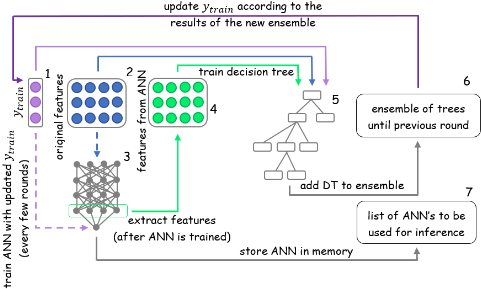
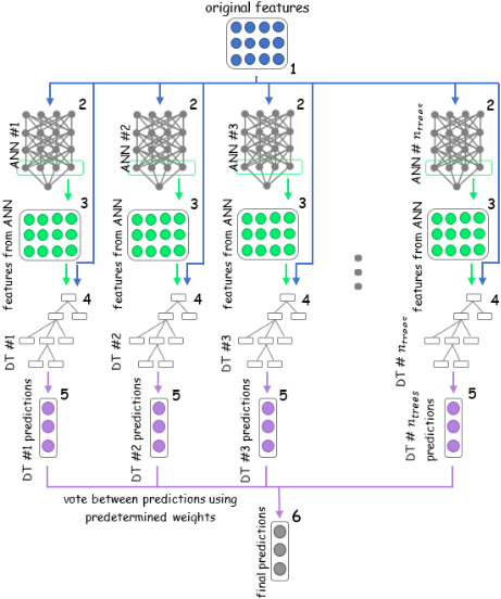
Clearly, this GBDT process assumes that {Xi}Ni=1 doesn't change throughout the training process. Theoretically, the features can be augmented between phases, and each individual function h can be trained on a different variation of these features. These augmentations will be represented by a series of functions {ft}Tt=1 , and the augmented features used in each iteration will be annotated ft(X). In the next sections we'll describe a number of methods for building {ft}Tt=1 : embedding the features using an ANN (AugBoost-ANN), and rotating the feature-space using PCA (AugBoost-PCA) or RP (AugBoost-RP). First we'll present diagrams which describe the phases of AugBoost-ANN during one iteration (AugBoost-PCA and AugBoost-RP can be described by similar figures). Second, we'll discuss the different methods for augmenting the features during each iteration. Finally, we'll present the complete pseudo-code of the training process.
In Figure 1, we present one iteration of AugBoost-ANN's training. The original features (#2 in the figure) are fed to the ANN (#3), which learns the updated target (#1), as presented in Equation 6. Then, a new set of features (#4) are extracted from the output of the ANN's last hidden layer, and concatenated with the original features (#2). The concatenated features are fed to a DT (#5), which learns the same updated target (#1) which the ANN used. This ANN is appended to the list of ANNs to be later used for inference (#7), and the DT is added to the ensemble of DTs (#6), together with a corresponding weight, to be used during inference. Finally, the loss of the updated ensemble is calculated, and this is used to update the target.
In Figure 2, we present the inference process of AugBoostANN. The original features (#1 in the figure), are fed to all of the ANNs (#2) which were trained on the training set. We then extract new features (#3) from the outputs of the last hidden layers of these ANNs. The original features are concatenated with the newly extracted ones, and each set of concatenated features is fed to a DT (#4). The DT and the ANN of each "branch" in the diagram were trained in the same iteration, during the training phase. We obtain predictions from each DT (#5), and we calculate a weighted sum using the weights learned during training.
2.2 Feature Extraction with ANNs
An ANN can be used to learn an embedding of the original features, which extracts and emphasizes the most "useful" information in the original features. The features are extracted using the following method:
- Train a neural network with the original features and their corresponding target.
- Select one of the hidden layers to extract the features from (usually one of the last hidden layers).
- Derive a "partial" neural network from the trained ANN, in which the layers following the selected hidden layer are dumped.
- To extract features for a new sample, use the standard prediction procedure of the partial ANN.
This process follows one of the most practical approaches for performing transfer learning in neural networks [Pan et al., 2010]: the first number of layers from a trained ANN are frozen, and then the rest of the layers are retrained on new data. The number of layers which are replaced is usually between 1-3, and depends on the amount of data for transfer learning and the similarity between the new task and the task of the original ANN. Instead of retraining the non-frozen layers, they can be replaced by any model (e.g. a decision tree). This suggests that the ANN embedding is effectively a lossy representation of the original data. However, if the complete ANN achieves good prediction performance, this indicates that the relevant information for the given task is at least somewhat preserved by the embedding. This potentially facilitates the training of a subsequent model, i.e. of a model that uses the embedded features as input, in comparison with the training using the original features representation.
In transfer learning, we assume that since the new task is similar to the original task, the embedding will be useful for the new task as well. When both tasks are identical, this is clearly the case, and therefore it is sensible to keep as many layers as possible from the trained ANN. This suggests that when the tasks are identical, we only dump the last layer of the ANN. Therefore, we follow [Chen et al., 2018] and extract features from the last hidden layer.
In order to augment the features in between iterations of the GBDT, we train an ANN until the loss ceases to improve, with the original features and the updated target (as in Equation 8). For each sample, the original features are fed as input to the ANN, and then concatenated with the features extracted from the last hidden layer. The next DT will be trained using this concatenation of features, and the updated targets.
2.3 Rotation of the Feature-Space with PCA or RP
Another approach towards augmenting the features in between iterations of GBDT, is by an unsupervised rotation of the feature space. Given a set of features and their corresponding targets {(Xi, yi)}Ni=1 , we wish to rotate {Xi}Ni=1 without loss of information, and with some randomization to generate diversity between the different rotations. We achieve this using two different approaches: PCA and RP.
For the PCA approach, we use a procedure similar to Rotation Forest [Rodriguez et al., 2006]: features are split into a number of random subsets, and then PCA is applied separately on each subset without dimensionality reduction (all of the PCA components are maintained). According to [Rodriguez et al., 2006], this rotation technique is meant as a diversifying heuristic, and not for finding good discriminatory directions. In addition to ensuring diversity among the trees, rotated trees also relax the constraint of univariate trees which are capable of splitting the input space only into hyperplanes that are parallel to the original feature axes. Moreover, another possible effect of this technique is a migration of information to the first components of each PCA procedure. PCA concentrates much of the variance in a few of the components, and this may indicate that these few components contain more information than we could expect from a subset of the original features (of the same size). These features can be exploited by some models, such as DTs, to obtain better results, for example by creating more compact trees which may help avoid overfitting. This is due to the fact that more features which are more informative may allow using less splits to represent a given decision rule. Unlike in Rotation Forest, we do not replace the original features with the new features, and instead we concatenate the two sets of features.
For the RP approach, we use a method similar to RPBoost [Casale et al., 2011] with a number of changes. First, we apply the projections separately on each of the randomly selected feature subsets (as in AugBoost-PCA), rather than projecting all of the features with the same RP. Second, we concatenate the original features and the new features (as in AugBoost-PCA), rather than only using the new features. Finally, we only re-augment the features once every number of iterations (we will elaborate on this in Section 2.4).
AugBoost-PCA and AugBoost-RP can also be described by Figures 1,2, except that the ANNs in the diagrams (#3 and #2 in Figures 1 and 2, respectively) are replaced by a pipeline which includes splitting the features into subsets and applying PCA or RP to each subset (ANN-embeddings can also be created seperately for each feature subset). Unlike an ANN, PCA and RP are unsupervised, and therefore don't receive the target as one of its' inputs during training.
2.4 Implementation Specifics
In order to compare the results of AugBoost 1 with the classic GBDT, we added a number of modules to the implementation of GBDT by scikit-learn[Pedregosa et al., 2011]. All comparisons were done with the default hyper-parameters of the existing libraries, and all hyper-parameters in the modules added by us were given a default value (which was used in all of the experiments). Since GBDT for classification consists of regression DTs, all neural networks that we trained solved regression problems (and used MSE as their loss function). Similarly, for classification tasks we applied PCA or RP separately for each class.
1 Code repository: https://github.com/ptannor/augboost
The ANNs had a simplistic and generic architecture, which was chosen using known best practices: three fully-connected hidden layers of the same size. The number of neurons in each of the hidden layers was defined to be the size of the input. The hidden layers all had ReLU activation functions, the output layer had a linear activation function. Batch size was chosen to be theminimumbetween 300 samples and 1 15 of the data. A random 15% of the training data was set aside for validation during the training of each ANN, and early stopping occurred if the validation loss didn't improve for 10 epochs. For all methods, the number of feature subsets is set by default to three (which are randomly chosen). PCA is applied separately on each subset of features, and none of the components of the PCA are dumped. Similarly, ANN-embeddings and RP maintain the dimension size of each feature subset. This practice is based on preliminary experiments, and for RP also on results from previous work [Casale et al., 2011].
Features were normalized by quantile normalization before applying any feature-augmentation method. The new features were concatenated with the original features before being used as the input for a DT (for training and inference). The concatenation technique is meant to utilize the new features, while also enabling the usage of the original features (which are carefully handcrafted by human experts in some cases). For practical reasons, the PCA-based transformation is typically calculated based only on the training set (this enables inference on a new test set without re-training the model).
In all of these methods, the training of the model used for feature augmentation isn't necessarily done during every iteration. Every nBA iterations we retrain the model, starting from the first iteration. In the rest of the iterations the model from the preceding iteration is duplicated (BA stands for 'Between Augmentations'). This is meant to enable the boosting process to exploit the information in each set of new features, since each individual DT may only be able to utilize a fraction of this information. Another advantage of this practice is that when the feature augmentation technique has significant computation costs, this is approximately nBA times faster than augmenting the features during each iteration. For most of our experiments, we used nBA = 10 and 150 iterations, i.e. we trained 150 DTs, and augmented the features 15 times throughout the process. In order to run experiments with RPBoost, we used our code for AugBoost-RP with a number of changes: nBA was set to be 1, the number of feature subsets was set to 1, and the original features weren't given as input to the decision trees (during both training and inference).
3 AugBoost Pseudo Code
In Algorithm 1 we present the training procedure, for all three of the augmentation methods. The presented procedure deals with the case of a regression task. In the case of a classification task, this procedure is conducted for each one of the classes, while the target is either 0 or 1 for each sample. To
Algorithm 1 AugBoost Training
Input: a training set {Xi, yi}Ni=1
Output: a model MT (X), which is based on T decision trees with their corresponding weights, and T augmentation functions
1: function TRAIN({Xi, yi}Ni=1) 2: Initialize M0(X) as argmin ρ ∑Ni=1 L(yi, ρ) ▷ L is the loss 3: Initialize { ˜ yi}Ni=1 as {yi}Ni=1 4: for t ← 1 to T do 5: if t - 1 is divisible by nBA then 6: Split the features of {Xi}Ni=1 to K random subsets. St,k def = func. that selects the features of subset k 7: For 1 ≤ k ≤ K, create a feature augmentation function ft,k for St,k(Xi) 8: else 9: For 1 ≤ k ≤ K: ft,k ← ft-1,k, St,k ← St-1,k 10: Update the targets {˜ yi}Ni=1 using the last gradient of L: - [ ∂L(yi ,M(Xi )) ∂M(Xi) ]M(X)=Mt-1(X) 11: Train a decision tree Dt, using {⋃Kk=1 (ft,k(St,k(Xi))), ˜ yi}Ni=1 12: Set ρt, the weight of the newmodel, to be argmin ρt ∑Ni=1 L(yi, Mt-1(Xi) +ρt · Dt(⋃Kk=1 (ft,k(St,k(Xi))))) 13: Mt(X) ←Mt-1(X) +ρt · Dt(ft(X))) 14: return MT (X)obtain the final predictions, the scores are later combined by weighted aggregation. The pseudo code is similar to GBDT, and the only differences are in the augmentations of the features marked ft. Initializations of the model ensemble and the target take place in lines 2-3. Lines 5-9 determine the augmentations to be used in the ensemble. Every nBA iterations the split into subsets and the augmentation functions are recalculated. For every other iteration, the augmentation function is copied from the preceding iteration, i.e. the augmentation function is only calculated once every nBA iterations. Line 7 determines if the algorithm is AugBoost-ANN, AugBoost-PCA or AugBoost-RP. If ft is the identity function, Algorithm 1 becomes the classic GBDT. Lines 10-14 are similar to the pseudo-code of the classic GBDT.
4 Experimental Results
We tested the classic GBDT (LightGBM implementation [Ke et al., 2017]), RPBoost, and all three versions of AugBoost on 20 classification datasets. The datasets [Dheeru and Karra Taniskidou, 2017; Alcala-Fdez et al., 2011] are from the UCI repository, Kaggle datasets, and the Keel dataset repository. As indicated in Table 1, the datasets vary across number of samples, number of features and number of classes. We performed 10-fold cross-validation and reported the mean cross-entropy.
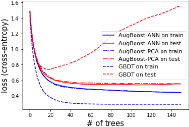
All of the AugBoost methods typically had less steep learning curves than GBDT on the training data, although in many cases they were better at generalizing (an example is presented in Figure 3).
In Table 1 we present comparisons between results of Aug- Boost methods, and the results of the classic GBDT (LightGBM implementation), over a wide range of datasets.
In 11 out of 20 cases, all three of the AugBoost methods outperfomed LightGBM. RPBoost is outperformed by all three versions of AugBoost on 15 out of 20 tasks. We used the Friedman test for validating the statistical significance of differences between the evaluated methods [Demˇsar, 2006]. The null-hypothesis that all five algorithms perform the same and the observed differences are merely random was rejected with FF (4, 76) = 17.88 and p < 0.01.
We proceeded with Nemenyi post-hoc tests, to conclude the following: AugBoost-ANN and AugBoost-PCA significantly outperform LightGBM with p < 0.05 and p < 0.1, respectively. AugBoost-ANN and AugBoost-PCA significantly outperform RPBoost with p < 0.05, and AugBoost-RP outperforms RPBoost as well with p < 0.1 (and is better on 18 out of 20 tasks).
We also examined the results of a single ANN, and of scikit-learn's implementation for the classic GBDT (which our code is based on), using the same hyperparameter settings. These aren't presented in table 1 since their performances were significantly inferior: the ANN was the worst performer for all of the tasks and scikit-learn's GBDT was inferior to LightGBM in 18 out of the 20 tasks (and the worst performer in 16 of the tasks).
5 Discussion
It is evident in the results that for classification tasks, the classic GBDT can be significantly improved by stage-wise feature augmentation. RPBoost seems to perform similarly to LightGBM, even though it is based on the code of scikitlearn, and is therefore "a step in the right direction". However the AugBoost methods which we proposed seem to outperform GBDT with higher statistical significance (while differences between versions of AugBoost have much lower statistical significance). This implies that although the choice of the augmentation method does seem to impact the results, it is not the only important component of our method. The main other components that seem to contribute to the results are: concatenating the augmented features with the original features, applying the chosen transformation on disjoint subsets of the features, and "recycling" each new set of augmented features for a number of iterations.
| dataset | # samples | # features | # classes | loss (cross-entropy) | ||||
|---|---|---|---|---|---|---|---|---|
| AugBoost-ANN | AugBoost-PCA | AugBoost-RP | RPBoost | LightGBM | ||||
| cortex (mice protein) | 1080 | 80 | 8 | 1.04E-3 ± 2.37E-4 | 5.79E-3 ± 8.57E-2 | 1.68E-2 ± 9.29E-3 | 9.71E-2±9.05E-3 | 1.75E-3 ± 4.34E-3 |
| CRX (credit approval) | 690 | 570 | 2 | 4.02E-1 ± 6.12E-2 | 3.23E-1 ± 4.76E-2 | 3.65E-1 ± 4.89E-2 | 3.73E-1±3.69E-2 | 4.83E-1 ± 1.45E-1 |
| nursery | 12960 | 8 | 5 | 8.07E-2 ± 1.49E-2 | 7.09E-2 ± 3.18E-2 | 2.21E-1 ± 1.56E-2 | 4.38E-1±1.17E-2 | 1.71E+0 ± 1.67E+0 |
| heart disease | 270 | 28 | 2 | 4.42E-1 ± 1.39E-1 | 5.55E-1 ± 2.42E-1 | 4.00E-1 ± 1.56E-1 | 3.95E-1±1.31E-1 | 5.54E-1 ± 2.18E-1 |
| shuttle (statlog) | 43500 | 9 | 7 | 8.06E-4 ± 6.80E-4 | 9.21E-4 ± 6.35E-4 | 7.44E-4 ± 5.28E-4 | 5.29E-2±3.42E-3 | 6.35E+0 ± 5.66E+0 |
| wilt | 4339 | 5 | 2 | 2.55E-2 ± 1.56E-2 | 2.73E-2 ± 1.61E-2 | 2.78E-2 ± 2.04E-2 | 3.25E-2±1.17E-2 | 3.40E-2 ± 2.41E-2 |
| titanic | 891 | 8 | 2 | 4.34E-1 ± 4.36E-2 | 4.56E-1 ± 5.18E-2 | 4.35E-1 ± 4.47E-2 | 4.45E-1±3.56E-2 | 6.50E-1 ± 7.55E-2 |
| gender-by-voice | 3168 | 20 | 2 | 6.29E-2 ± 2.32E-2 | 6.06E-2 ± 2.55E-2 | 6.26E-2 ± 2.37E-2 | 1.66E-1±2.30E-2 | 8.89E-2 ± 5.17E-2 |
| adult | 32560 | 14 | 2 | 2.97E-1 ± 5.39E-3 | 2.88E-1 ± 5.40E-3 | 3.06E-1 ± 7.21E-3 | 3.78E-1±5.70E-3 | 2.77E-1 ± 4.74E-3 |
| frogs-MFCCs | 7195 | 22 | 10 | 6.87E-2 ± 1.29E-2 | 6.65E-2 ± 1.46E-2 | 7.18E-2 ± 1.58E-2 | 1.37E-1±1.63E-2 | 6.25E-2 ± 2.17E-2 |
| Wisconsin breast cancer | 569 | 30 | 2 | 1.06E-1 ± 1.00E-1 | 1.23E-1 ± 1.10E-1 | 1.12E-1 ± 1.04E-1 | 9.17E-2±4.83E-2 | 1.37E-1± 1.65E-1 |
| banknote authentication | 1372 | 4 | 2 | 1.32E-2 ± 1.69E-2 | 1.37E-2 ± 1.43E-2 | 1.38E-2 ± 1.43E-2 | 5.69E-2±1.20E-2 | 1.31E-2 ± 2.76E-1 |
| car evaluation | 1727 | 6 | 4 | 1.41E+0 ± 1.45E-2 | 1.31E+0 ± 3.13E-2 | 1.38E+0 ± 1.55E-2 | 1.44E+0±1.71E-2 | 1.62E+0 ± 5.01E-2 |
| CTG data (cardio) | 2126 | 35 | 3 | 4.08E-2 ± 2.28E-2 | 5.20E-2 ± 2.99E-2 | 4.90E-2 ± 2.01E-2 | 9.37E-2±1.38E-2 | 7.86E-2 ± 4.66E-2 |
| contraceptive method | 1472 | 9 | 3 | 9.25E-1 ± 3.13E-2 | 9.38E-1 ± 3.28E-2 | 9.47E-1 ± 2.22E-2 | 9.55E-1±1.51E-2 | 1.08E+0 ± 5.84E-2 |
| messidor (diabetes) | 1151 | 19 | 2 | 5.68E-1 ± 2.26E-2 | 5.70E-1 ± 3.60E-2 | 5.82E-1 ± 1.54E-2 | 6.12E-1±2.36E-2 | 6.89E-1 ± 7.69E-2 |
| parkinson | 1040 | 27 | 2 | 2.98E-4 ± 5.00E-6 | 2.95E-4 ± 4.89E-7 | 2.98E-4 ± 8.00E-6 | 1.44E-1±1.80E-2 | 2.00E-6 ± 3.10E-9 |
| pen digits | 7494 | 16 | 10 | 4.39E-2 ± 1.05E-2 | 3.17E-2 ± 8.29E-3 | 5.32E-2 ± 5.68E-3 | 1.47E-1±1.39E-2 | 3.15E-2 ± 1.11E-2 |
| phishing | 1353 | 9 | 3 | 3.03E-1 ± 4.67E-2 | 2.46E-1 ± 4.46E-2 | 2.93E-1 ± 3.45E-2 | 3.55E-1±2.27E-2 | 3.08E-1 ± 9.51E-2 |
| flare | 1066 | 11 | 6 | 5.77E-1 ± 8.80E-2 | 6.67E-1 ± 1.12E-1 | 5.61E-1 ± 7.57E-2 | 5.83E-1±7.60E-2 | 7.03E-1 ± 1.48E-1 |
| average ranking | 2.25 | 2.5 | 2.65 | 3.9 | 3.7 | |||
nBA is a crucial parameter, and it essentially determines how many iterations follow each augmentation of the features. If nBA = 1, runtime is fairly long (especially for the case of AugBoost-ANN), and the boosting process may not get a chance to exploit important information for the augmented features. If nBA is too large, we could expect an ensemble with lower diversity. Therefore, nBA should be chosen carefully to assume a value which would balance these two considerations.
Preliminary experiments demonstrated that dimensionality reduction doesn't improve the results, for any of the augmentation methods. Increasing the dimensionality with a ANN may enable an improvement in accuracy results, similarly to good feature extraction. Utilizing more features in an efficient manner may require more iterations, and possibly more spacing between feature augmentations. This can be further explored, although PCA cannot increase the dimensionality by definition and from the results of Cascale et al. [Casale et al., 2011], it seems that increasing the dimensionality with RP may damage the accuracy results significantly. This may be due to the fact that each individual feature doesn't contain enough information to facilitate meaningful splits in the DTs.
6 Conclusions and FutureWork
In this paper, we presented different methods for enhancing the performance of GBDT by augmenting the features in between iterations, and concatenating the new features with the original ones before training each new DT. Even though these methods they are fairly different one from another, they all significantly outperform the classic GBDT (scikit-learn implementation), and two of the tree methods significantly outperform LightGBM's implementation as well. This implies that further exploration of stage-wise feature augmentation methods may lead to even better results.
The work presented in this paper may very well be improved by further research. Primarily, the ANN architecture and hyper-parameters can be chosen with meta-learning techniques, and don't have to be chosen in a "one fits all" manner. This is especially important due to AugBoost-ANN's high time-complexity, which makes it difficult to tune hyperparameters. This may also be true for selecting the standard hyper-parameters of GBDT (which are inherited by AugBoost-ANN). Secondly, in each iteration we trained the DTs using the concatenation of the newly obtained features and original features. However, feature selection could be applied to the concatenated features before training each DT.
Furthermore, if we only the DTs with just the newly obtained features (rather than the concatenation of both sets of features), we may be able to use AugBoost-ANN on more complex data such as: images, text, audio, etc (while using more complex ANN architectures). This could be useful for tasks such as fine-grained classification.
We've presented a number of methods for feature augmentation. Other methods could be explored as well, such as other automatic methods for feature extraction (unsupervised), the encoder from an auto-encoder ANN (unsupervised), TSNE (unsupervised) and LDA (supervised). Once a wide variety of techniques for this type of augmentation have been implemented, one could experiment with combinations of a number of techniques (i.e. using different feature augmentation methods in different iterations). The methods presented in this paper are also applicable for regression tasks, although obtaining good results on regression tasks may require some changes in the implementation specifics.
From a coding point of view, we based the code on scikit-learn's GBDT since it was simple to modify, and not because it performs best. Embedding AugBoost in other GBDT libraries (such as XGBoost[Chen and Guestrin, 2016], LightGBM[Ke et al., 2017] or CatBoost[Prokhorenkova et al., 2017]) may improve the results.
@inproceedings{ijcai2019p493,
  title     = {AugBoost: Gradient Boosting Enhanced with Step-Wise Feature Augmentation},
  author    = {Tannor, Philip and Rokach, Lior},
  booktitle = {Proceedings of the Twenty-Eighth International Joint Conference on
               Artificial Intelligence, {IJCAI-19}},
  publisher = {International Joint Conferences on Artificial Intelligence Organization},
  editor    = {Sarit Kraus},
  pages     = {3555--3561},
  year      = {2019},
  month     = {8},
  note      = {Main track},
  doi       = {10.24963/ijcai.2019/493},
  url       = {https://doi.org/10.24963/ijcai.2019/493},
}
TY - CPAPER TI - AugBoost: Gradient Boosting Enhanced with Step-Wise Feature Augmentation AU - Tannor, Philip AU - Rokach, Lior T2 - Proceedings of the Twenty-Eighth International Joint Conference on Artificial Intelligence, IJCAI-19 PB - International Joint Conferences on Artificial Intelligence Organization PY - 2019 SP - 3555 EP - 3561 DO - 10.24963/ijcai.2019/493 UR - https://doi.org/10.24963/ijcai.2019/493 ER -Copied
Machine-readable versions of this paper, for tools and AI agents:





