
Taming the Noisy Gradient: Train Deep Neural Networks with Small Batch Sizes
Proceedings of the Twenty-Eighth International Joint Conference on Artificial Intelligence. Main track. Pages 4348-4354.
https://doi.org/10.24963/ijcai.2019/604
Keywords
- Machine Learning: Deep Learning
- Machine Learning: Classification
Abstract
Deep learning architectures are usually proposed with millions of parameters, resulting in a memory issue when training deep neural networks with stochastic gradient descent type methods using large batch sizes. However, training with small batch sizes tends to produce low quality solution due to the large variance of stochastic gradients. In this paper, we tackle this problem by proposing a new framework for training deep neural network with small batches/noisy gradient. During optimization, our method iteratively applies a proximal type regularizer to make loss function strongly convex. Such regularizer stablizes the gradient, leading to better training performance. We prove that our algorithm achieves comparable convergence rate as vanilla SGD even with small batch size. Our framework is simple to implement and can be potentially combined with many existing optimization algorithms. Empirical results show that our method outperforms SGD and Adam when batch size is small. Our implementation is available at https://github.com/huiqu18/TRAlgorithm.
- [Allen-Zhu, 2018] Zeyuan Allen-Zhu. How to make the gra- dients small stochastically: Even faster convex and non- convex sgd. In Advances in Neural Information Process- ing Systems, pages 1165-1175, 2018.
- [Bottou, 2010] Léon Bottou. Large-scale machine learn- ing with stochastic gradient descent. In Proceedings of COMPSTAT'2010, pages 177-186. Springer, 2010.
- [Bottou, 2012] Léon Bottou. Stochastic gradient descent tricks. In Neural networks: Tricks of the trade, pages 421- 436. Springer, 2012.
- [Chaudhari et al., 2017] Pratik Chaudhari, Anna Choroman- ska, S. Soatto, Yann LeCun, C. Baldassi, C. Borgs, J. Chayes, Levent Sagun, and R. Zecchina. Entropy-sgd: Biasing gradient descent into wide valleys. In Interna- tional Conference on Learning Representations (ICLR), 2017.
- [Cordts et al., 2016] Marius Cordts, Mohamed Omran, Se- bastian Ramos, Timo Rehfeld, Markus Enzweiler, Rodrigo Benenson, Uwe Franke, Stefan Roth, and Bernt Schiele. The cityscapes dataset for semantic urban scene under- standing. In CVPR, pages 3213-3223, 2016.
- [Ge et al., 2015] Rong Ge, Furong Huang, Chi Jin, and Yang Yuan. Escaping from saddle points-online stochastic gra- dient for tensor decomposition. In Conference on Learning Theory, pages 797-842, 2015.
- [Hardt et al., 2016] Moritz Hardt, Ben Recht, and Yoram Singer. Train faster, generalize better: Stability of stochas- tic gradient descent. In International Conference on Ma- chine Learning, pages 1225-1234, 2016.
- [He et al., 2016] Kaiming He, Xiangyu Zhang, Shaoqing Ren, and Jian Sun. Deep residual learning for image recog- nition. In Proceedings of the IEEE conference on computer vision and pattern recognition, pages 770-778, 2016.
- [Hoerl and Kennard, 1970] Arthur E Hoerl and Robert W Kennard. Ridge regression: Biased estimation for nonorthogonal problems. Technometrics, 12(1):55-67, 1970.
- [Huang et al., 2017] Gao Huang, Zhuang Liu, Laurens Van Der Maaten, and Kilian Q Weinberger. Densely connected convolutional networks. In Proceedings of the IEEE con- ference on computer vision and pattern recognition, pages 4700-4708, 2017.
- [Isola et al., 2017] Phillip Isola, Jun-Yan Zhu, Tinghui Zhou, and Alexei A Efros. Image-to-image translation with con- ditional adversarial networks. In CVPR, pages 1125-1134, 2017.
- [Jin et al., 2017] Chi Jin, Rong Ge, Praneeth Netrapalli, Sham M Kakade, and Michael I Jordan. How to escape saddle points efficiently. In Proceedings of the 34th In- ternational Conference on Machine Learning-Volume 70, pages 1724-1732. JMLR. org, 2017.
- [Johnson and Zhang, 2013] Rie Johnson and Tong Zhang. Accelerating stochastic gradient descent using predictive variance reduction. In Advances in neural information pro- cessing systems, pages 315-323, 2013.
- [Kingma and Ba, 2014] Diederik P Kingma and Jimmy Ba. Adam: A method for stochastic optimization. In ICLR, 2014.
- [Le et al., 2011] Quoc V Le, Jiquan Ngiam, Adam Coates, Abhik Lahiri, Bobby Prochnow, and Andrew Y Ng. On optimization methods for deep learning. In Proceedings of the 28th International Conference on International Con- ference on Machine Learning, pages 265-272. Omnipress, 2011.
- [Lei and Jordan, 2017] Lihua Lei and Michael Jordan. Less than a single pass: Stochastically controlled stochastic gra- dient. In Artificial Intelligence and Statistics, pages 148- 156, 2017.
- [Lin et al., 2015] Hongzhou Lin, Julien Mairal, and Zaid Harchaoui. A universal catalyst for first-order optimiza- tion. In Advances in Neural Information Processing Sys- tems, pages 3384-3392, 2015.
- [Long et al., 2015] Jonathan Long, Evan Shelhamer, and Trevor Darrell. Fully convolutional networks for seman- tic segmentation. In CVPR, pages 3431-3440, 2015.
- [Parikh et al., 2014] Neal Parikh, Stephen Boyd, et al. Prox- imal algorithms. Foundations and Trends R in Optimiza- tion, 1(3):127-239, 2014.
- [Rakhlin et al., 2012] Alexander Rakhlin, Ohad Shamir, and Karthik Sridharan. Making gradient descent optimal for strongly convex stochastic optimization. In Proceedings of the 29th International Coference on International Confer- ence on Machine Learning, pages 1571-1578. Omnipress, 2012.
- [Reddi et al., 2016] Sashank J Reddi, Ahmed Hefny, Suvrit Sra, Barnabas Poczos, and Alex Smola. Stochastic vari- ance reduction for nonconvex optimization. In Interna- tional conference on machine learning, pages 314-323, 2016.
- [Reddi et al., 2018] Sashank J Reddi, Satyen Kale, and San- jiv Kumar. On the convergence of adam and beyond. In ICLR, 2018.
- [Ruder, 2016] Sebastian Ruder. An overview of gradi- ent descent optimization algorithms. arXiv preprint arXiv:1609.04747, 2016.
- [Shamir and Zhang, 2013] Ohad Shamir and Tong Zhang. Stochastic gradient descent for non-smooth optimization: Convergence results and optimal averaging schemes. In International Conference on Machine Learning, pages 71- 79, 2013.
- [Wang et al., 2018] Ting-Chun Wang, Ming-Yu Liu, Jun- Yan Zhu, Andrew Tao, Jan Kautz, and Bryan Catanzaro. High-resolution image synthesis and semantic manipula- tion with conditional gans. In Proceedings of the IEEE Conference on Computer Vision and Pattern Recognition, pages 8798-8807, 2018.
References were extracted automatically from the PDF and may contain errors.
Full text extracted automatically from the PDF; figures, tables and equations may differ. The PDF is the version of record.
1 Introduction
Recent years have witnessed the rapid development of deep neural networks in a wide range of applications. The success of neural networks should be partially attributed to optimization algorithms such as stochastic gradient descent (SGD) and its variants [Kingma and Ba, 2014]. These popular optimization methods, widely adopted in practice, have been proved to be extremely efficient and effective for finding the local minima of the objective function [Bottou, 2010; Bottou, 2012; Le et al., 2011]. SGD exploits the finite sum structure of the objective function, avoids the expensive computation of exact gradient, and thus provides a feasible and efficient optimization solution in practice [Bottou, 2012]. The stochastic nature also helps escaping saddle points, when Newton method cannot [Ge et al., 2015; Jin et al., 2017]. It has also been shown both empirically and theoretically that SGD and its variants improve the generalization performance of the trained models [Hardt et al., 2016; Chaudhari et al., 2017].
∗ equal contribution
Despite the above advantages, one limitation with SGD type methods has manifested in recent years. Calculated using partial data, the stochastic gradient tends to fluctuate [Ruder, 2016] and deviate from the full gradient descent direction, causing deteriorated optimization efficiency. This issue becomes more serious when researchers continuously develop powerful yet large size networks to address big data challenges. With large networks, we are often forced to use small batch size due to the memory constraints. For example, in the high resolution image synthesis task [Wang et al., 2018], it requires a GPU of 24GB memory to train a generative adversarial network (GAN) using full resolution images with batch size 1. Such scenario demands small batch sizes, causing large variance in stochastic gradients, and thus inefficient optimization.
Variance reduction techniques have been developed to alleviate such issue [Johnson and Zhang, 2013; Reddi et al., 2016; Lei and Jordan, 2017]. These techniques reduce the noise of stochastic gradient by progressively estimating the difference between noisy and noiseless gradient. However, these techniques require the access to gradient computed by full batch or large batch size, and thus is impractical in the limited memory/small batch size scenario.
In this paper, we propose a new optimization method to reduce the variance of stochastic gradients with small batch size. Our method, called Trajectory Regularized Algorithm (TRAlgo), computes each stochastic gradient by locally adding a proximal type regularizer. The locally regularized loss function becomes strongly convex and can be solved efficiently [Rakhlin et al., 2012]. The local regularizer stabilizes the stochastic gradient, and thus reduces its variance. We prove that with small batch size, our method can achieve a much better stochastic gradient variance compared with SGD, and thus a better convergence rate. Our algorithm is fairly general and in principle can be combined with many existing SGD type methods. It opens the door toward novel optimization techniques that uniquely suit the big data world. In summary, our main contributions include:
- We propose a new algorithm using proximal regularizer to address the issue of noisy stochastic gradients, due to small batch size.
- We prove that our algorithm converges no slower than SGD. Furthermore, under the constraint of small batch size, our method reduces the variance of stochastic gradients, and thus has a better convergence rate than SGD.
- We combine our algorithm with various state-of-the-art optimization algorithms (vanilla SGD and Adam). We empirically show that the proposed method improves the optimization performance when training deep neural networks with small batch sizes.
Note that the power of a proximal type regularizer has been exploited [Allen-Zhu, 2018; Lin et al., 2015]. However, existing works only focus on the optimization efficiency. To the best of our knowledge, TRAlgo is the first to use such technique to address noisy gradients, under the small batch size constraint.
The remainder of this paper is organized as follows. We introduce our notation and TRAlgo in Section 2. In Section 3, we combine TRAlgo with SGD (called TRSGD) and analyze the gradient complexity of both TRSGD and SGD. Experimental results are presented in Section 4. Finally, we conclude our work in Section 5.
2 Preliminary
We introduce the notations, assumptions, as well as our proposed TRAlgo framework. Throughout this paper, we denote by f(w) = 1n ∑ni=1 fi(w) the loss function, where w ∈ Rd represents parameters in the optimization problem. We use ‖ · ‖ to denote the L2 norm. In this paper, we only consider convergence to a first order stationary point : ‖∇f(x)‖2 ≤ ϵ.
The following assumptions are widely adopted in the analysis of convex and non-convex optimization algorithms. They regulate the behavior of zero-th order, first order and second order derivatives of f(x).
Assumption 1. We assume following conditions hold:
- Function f(x) is ℓ-Lipschitz smooth: ‖∇f(x) - ∇f (y)‖ ≤ ℓ‖x - y‖.
- Function f(x) is G-Lipschitz continuous: ‖f(x) - f (y)‖ ≤ g‖x - y‖.
- Function f(x) is B bounded: |f(x)| ≤ B
In following assumption we apply δ to describe how 'nonconvex' f(x) is.
Assumption 2 (δ-non-convex). We assume function f(x) is δ-non-convex : f (x) ≥ f (y) + 〈∇f (y), x - y〉 - δ2 ‖y - x‖2
In general, δ is uniformly bounded by Hessian upper bound ℓ and could be equivalent to ℓ in the worst case. We can view δ as the minimum value of λ so that f(w)+ λ2 ‖w‖2 is convex.
Assumption 3 (Variance bounded SGD). We assume function f(x) is σ variance bounded: 1n ∑ni=1 ‖∇fi(w) - ∇f(w)‖2 ≤ σ2 .
The last assumption regulates the variance of stochastic gradient which is common in analyzing the convergence behavior of Stochastic Gradient Descent.
Algorithm 1 presents our Trajectory Regularized framework. It run for T iterations. At iteration t, we will construct
Algorithm 1 TRAlgo (T, λ, w0, S)
- 1: Input: Number of iterations T, Regularizer weight λ, Initialization w0
- 2: for t = 0, · · · , T -1 do
- 3: Gt(w) = f(w) + λ2 ‖w-wt‖2
- 4: Run stochastic gradient type method with decreasing step size on Gt(w) for S iterations to compute wt+1
- 5: Option I:
- 6: Pick ˆw = wT
- 7: return ˆw
▷ In practice
- 8: Option II:
- 9: Pick ˆw uniformly randomly fromw1, ..,wT
- 10: return ˆw
▷ For analysis
an auxiliary function Gt(w) by adding a regularization term to f(x), and run stochastic gradient type optimization algorithm on Gt(w) for S iterations. The result w after S steps is the next gradient step, wt+1. After T iterations, depending on the context, we may return wT as the final output (in practice), or return a random sample from all previous w∗ (for analysis).
The key idea of TRAlgo is to apply a proximal type regularizer λ2 ‖w - wt‖2 with λ ≥ 2δ to make the loss function f(x) strongly convex. The regularizer stablizes the gradient and thus reduces its variance, as we will prove in the next section. To avoid introducing bias as a fixed regularizer does [Hoerl and Kennard, 1970], the regularizer is locally adaptive (centered at current wt). Quadratic proximal regularizer has been used before [Parikh et al., 2014], but only for better optimization of non smooth L1 loss function. Instead, TRAlgo uses the it for a trajectory regularization purpose. In TRAlgo, the choice of the stochastic gradient method in each iteration is flexible. One can apply a vanilla SGD or its variants: Adam [Kingma and Ba, 2014] and AMSGrad [Reddi et al., 2018]. In next section, we use SGD as an example to analyze the benefits of TRAlgo, while in Section 4, we empirically apply TRAlgo to both SGD and Adam.
3 Analysis
In this section we incorporate SGD into our framework TRAlgo (called TRSGD) and compare it with Vanilla SGD. In Section 3.1 we review SGD and restate some known results of SGD for a direct comparison with analysis for TRSGD. In Section 3.3 we formally define TRSGD and analyze its convergence rate using batch size 1. While TRSGD achieves comparable gradient complexity with Vanilla SGD in general it attains a better convergence rate when batch size is constrained. The analysis focuses on quantifying how number of iterations S run on auxiliary function Gw(w) affects the convergence. Our analysis demonstrates even when batch size is limited, TRSGD could still control variance.
3.1 SGD
In Algorithm 2 we describe the Stochastic Gradient Descent method. We use I k ⊂ [n] to denote the random sampled
Algorithm 2 SGD(S, w0, η0:S-1)
- 1: Input: Number of iterations S; Initial valuew0; Step size η0:S-1
- 2: for k = 0, · · · , S -1 do
- 3: wk+1 = wk - ηk∇fIk (wk)
- 4: Option I:
- 5: Pick ˆw = wS
- 6: return ˆw
▷ For practice
- 7: Option II:
- 8: Pick ˆw uniformly randomly fromw1, ..,wS
- 9: return ˆw
▷ For analysis
small batch and ∇fIk (wk) = 1 |Ik | ∑i∈Ik ∇fi(wk) to denote the stochastic gradient in k-th iteration. The SGD update step is wk+1 = wk - ηk∇fIk (wk). Compared to full gradient update wk+1 = wk - ηk∇f(wk), the difference ∇fIk (wk) - ∇f(wk) is known as noise in stochastic gradient. Next we introduce some well known results about the convergence behavior of SGD and demonstrate how the noise affects the convergence. One can find similar statements in [Allen-Zhu, 2018; Ge et al., 2015; Reddi et al., 2016].
Lemma 1. Under assumptions 1 and 3, the iterative update of SGD with step size η ≤ 1 2ℓ and batch size M satisfies the following inequality:
Proof: By smoothness of f(x) we have f(wt+1) ≤ f(wt) + 〈∇f(wt),wt+1 - wt〉 + ℓ2 ‖wt+1 - wt‖2 . Recall that the SGD update rule is wt+1 = wt - η(∇f(wt) + σt) where σt represents noise in the Stochastic Gradient with E [σt] = 0, E [‖σt‖2 ] ≤ σ2 M . We have:E [f(wt+1)|wt] ≤ f(wt) + E [〈∇f(wt),wt+1 -wt〉 + ℓ2 ‖wt+1 -wt‖2 ] ≤ f(wt) - η‖∇f(wt)‖2 + ℓη2 2 ‖∇f(wt) + σt‖2 ≤ f(wt) - η2 ‖∇f(wt)‖2 + ησ2 4M .
3.2 Intuition: Noisy Gradient Slows Down Convergence
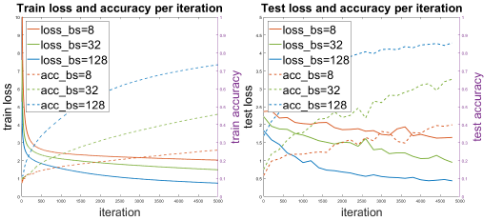
The left hand side of Eq. (1) is the improvement made in each iteration in expectation and the right hand side gives a guarantee on the progress for iteration t. One can observe that large variance will slow down the improvement brought by gradient. To alleviate this issue, one may increase batch size M. However, in our setting, when M is restricted to small, we cannot mitigate the negative impact of variance. Such phenomenon is shown in Figure 1.
By telescoping Lemma 1 and using the fact that f(x) - f(y) ≤ 2B, we have the convergence rate of SGD.
Theorem 1. Under assumptions 1 and 3, for SGD with step size η = 1/(2ℓ), batch size M, and any T , it holds that:
In particular, denote by N = TM the total number of gradient calls applied in the algorithm, picking T = 4√ℓBN/σ, the gradient complexity to reach E [‖∇f(w)‖2 ] ≤ ϵ is: N = O ( 1 ϵ2 ).
Above Theorem suggests that if picking the output of SGD uniformly randomly over w1:T , one can achieve E [‖∇f (w)‖2 ] = O ( ℓB T + σ2 T N ) . One could increase training iteration T and batch size M so that the expected gradient squared norm meets the first order stationary point criterion. An optimal choice balancing (ℓB) /T and (σ2T ) /N would be T = 4√ℓBN/σ. Although the above statements reveal the power of SGD in efficiency, it is not realistic to set M = Ω(√N) in training large size deep neural network.
Indeed, in the practical setting we are addressing, M may be a small constant (say 1). The right hand side of Eq. (2) can be arbitrarily bad with noisy gradients. In next section, we will show how TRAlgo addresses the issue and still keep a tight bound even with M = 1.
3.3 TRSGD
Our method TRAlgo requires the choice of a base optimization algorithm. In this section, we instantiate our method using the Vanilla SGD. We analyize the convergence performance of this instantiation, called TRSGD.
Definition 1. TRSGD is defined as applying SGD in TRAlgo: wt+1 = SGD(S,wt, ηk = 1/((λ - δ)k)) where k ∈ [S] represents k-th iteration in SGD.
While the advantage of decreasing stepsize (usually set to be 1/k) for SGD type methods has been well studied in strongly convex case [Rakhlin et al., 2012; Shamir and Zhang, 2013], it remains unclear how to properly apply such strategy in non-convex stochastic optimization. In the rest of this section we show one can benefit from such strategy due to the convexity of auxiliary function Gt(w).
First we state a technical lemma which follows [Rakhlin et al., 2012]. We use the following lemma to quantify the progress made by running SGD for S iterations with decreasing step size.
Lemma 2. If one runs SGDonGt(w) = f(w)+ λ2 ‖w-wt‖2 for S iterations with step size ηk = 1/((λ - δ)k) and batch size 1, one have ‖wt+1 - w∗ t+1 ‖2 ≤ 4(λ+ℓ)2 (g+σ2 ) (λ-δ)2 S where w∗ t+1 = arg minw{Gt(w)}.
| Method | CIFAR10 | CIFAR100 | ||||
|---|---|---|---|---|---|---|
| ResNet18 | ResNet101 | DenseNet121 | ResNet18 | ResNet101 | DenseNet121 | |
| SGD | 0.9467 | 0.9383 | 0.9390 | 0.7625 | 0.7439 | 0.7499 |
| TRSGD | 0.9522 | 0.9560 | 0.9537 | 0.7811 | 0.8008 | 0.8001 |
| Adam | 0.9250 | 0.9146 | 0.9242 | 0.7235 | 0.6918 | 0.7226 |
| TRAdam | 0.9453 | 0.9466 | 0.9472 | 0.7599 | 0.7812 | 0.7773 |
Now we are ready to prove the key lemma which describes one round progress of TRSGD. One can make a direct comparison between the following lemma and Lemma 1 by setting η = 1/(2ℓ) in Eq. (1).
Lemma 3. Under assumptions 1, 2 and 3, the iterative update of TRSGD with λ = 2ℓ and batch size 1 satisfies the following inequality:
While in Eq. (1) the issue of variance could be alleviated by increasing the batch size M for SGD, one can alleviate such issue by increasing the number of iterations S in Eq. (3) for TRSGD. One can set S = Θ(M) so both algorithms have a comparable one round convergence progress. However, in practice the choice of M is limited due to the memory restriction but the choice of S is not. We choose batch size to be 1 for simplicity and the analysis can be generalized to any batch size.
We finish this section by telescoping Eq. (3) to derive the following theorem. The inequality bounds the expected squared norm of gradient of TRSGD, similar to Theorem 1.
Theorem 2. Under assumptions 1, 2 and 3, the TRSGD with batch size 1 , λ = 2ℓ achieves the following convergence rate:
In particular, let N = TS be the total number of gradient call applied in the algorithm, by picking T = 4√BN/√ℓ(σ2 + g2 ), the gradient complexity to reach E [‖∇f(w)‖2 ] ≤ ϵ is N = O ( 1 ϵ2 ).
By setting the batch size to be 1, the gradient complexity of TRSGD is comparable to SGD in a rate of N = O (1/ϵ2 ) to meet the criterion E [‖∇f(wt)‖2 ] ≤ ϵ.
Interpretation of theorems. We can now explicitly compare Eq. (4) and Eq. (2). While the function loss term ℓB/T appear in both inequality the σ2 term appears in different fashion due to their strategies in monitoring variance. When gradient is associated with big variance, SGD increases batch size M and TRSGD runs more iteration on auxiliary function Gt(w). The strategy of TRSGD is not restricted by memory which is adorable in training huge network. The choice of S depends on the batch size restriction. In the case where one only affords to set M = 1, one can take S = Θ(√N) to optimally balance ℓB/T and (ℓ2 (σ2 + g2 )T)/N in the gradient complexity. On another hand, when it is possible to set M = Θ(√N), the TRAlgo framework will not be the first choice as there is no need for variance control.
4 Experiments
In this section we apply the proposed framework to momentum SGD and Adam algorithms, called TRSGD and TRAdam, respectively, and empirically illustrate the effectiveness of our methods when training deep neural networks with small batch sizes. We first compare the performance of different algorithms on image classification tasks on CIFAR10 and CIFAR100 datasets, and then show the application of our framework in the training of GANs using an image to image translation task on the Cityscapes dataset [Cordts et al., 2016]. We also perform ablation study on the batch size and iteration number S on TRSGD.
4.1 Implementation Details
Image classification. Three different deep neural networks are adopted in the image classification tasks: ResNet18 [He et al., 2016], ResNet101 [He et al., 2016] and DenseNet121 [Huang et al., 2017]. Four algorithms (TRSGD, SGD, TRAdam, Adam) are used to train these networks on CIFAR10 and CIFAR100. In all experiments, the number of epoch is 200 and the batch size is 8. For TRSGD and SGD, the momentum is 0.9, the learning rate is initially set to 0.1 and decayed to 0.01, 0.001 at epoch 100 and 150, respectively. For TRAdam and Adam, β1 = 0.9, β2 = 0.999, the learning rate is initially set to 0.001 and decayed to 0.0001, 0.00001 at epoch 100 and 150, respectively. For both TRSGD and TRAdam, λ = 0.1 and S = 10.
Image to image translation using GAN. In this task we follow the network structure and parameter settings of [Isola et al., 2017] to train a model that generates images from semantic labels on Cityscapes dataset. The only difference is that we replace the Adam optimizer with our TRAdam algorithm. In TRAdam, λ = 0.1, S = 10 and the other parameters are the same as Adam.
4.2 Results
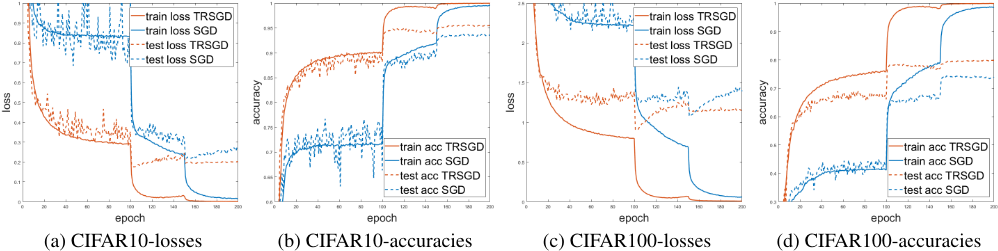
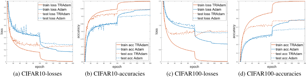
Image classification. The train and test curves of SGD vs. TRSGD, and Adam vs. TRAdam using a batch size of 8 are shown in Fig. 2 and Fig. 3, respectively. Only results of ResNet101 are presented due to the space limitation. We can observe that our TRSGD and TRAdam achieve faster convergence and better accuracies compared to SGD and Adam on both datasets. The test accuracies of all models are reported in Table 1. It is evident that our TRSGD and TRAdam outperform SGD and Adam in all cases. Because of the large gradient variance when the batch size is small, SGD and Adam are not able to obtain better performance with deeper networks. However, our algorithms can handle the noisy gradients by the regularizer, thus achieving higher accuracies using ResNet101 and DenseNet121, especially on CIFAR100 dataset.
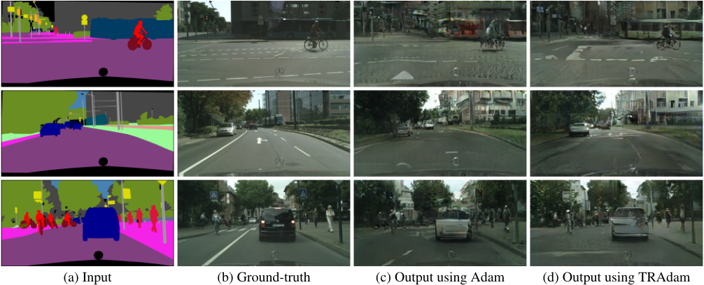
Image to image translation using GAN. To evaluate the image quality generated by the model, we use the "FCNscore" as in [Isola et al., 2017]. It evaluates how realistic the generated images are based on the semantic segmentation results using a pre-trained fully convolutional neural network. The pre-trained model predicts labels from the synthesized images. Then the labels are compared with the ground-truth labels those images were synthesized from. We adopt two pre-trained semantic segmentation models to compute "FCN-score": FCN-8s [Long et al., 2015] and DPCxception71 [Isola et al., 2017]. FCN-8s is used in Isola et al. [2017] while DPC-xception71 has the state-of-the-art performance on the Cityscapes dataset thus is more reliable than FCN-8s to compute the score. The evaluation results using two models are reported in Table 2 and Table 3. For the results evaluated by FCN-8, TRAdam is only slightly better in the per-pixel accuracy compared to Adam. However, TRAdam outperforms Adam in all three metrics when evaluated by DPC-xception71. The ground-truth metrics (GT in the tables) using original images for segmentation are also provided for reference. When computing the ground-truth values, we use the resized 256×256 version of original images because the resolution of synthesized images is 256×256. Some synthesized images are presented in Fig. 4.
| Method | Per-pixel acc. | Per-class acc. | Class IOU |
|---|---|---|---|
| GT | 0.70 | 0.26 | 0.19 |
| Adam | 0.64 | 0.24 | 0.17 |
| TRAdam | 0.66 | 0.24 | 0.17 |
4.3 Ablation Study
In this section we explore the effect of batch size and inner iteration number S on our TRSGD algorithm. ResNet18 and CIFAR10 dataset are used in all experiments of this section.
| Method | Per-pixel acc. | Per-class acc. | Class IOU |
|---|---|---|---|
| GT | 0.81 | 0.71 | 0.56 |
| Adam | 0.48 | 0.31 | 0.19 |
| TRAdam | 0.59 | 0.32 | 0.22 |
| Batch Size | 2 | 8 | 32 | 128 |
|---|---|---|---|---|
| SGD | 0.8569 | 0.9467 | 0.9518 | 0.9436 |
| TRSGD | 0.9131 | 0.9522 | 0.9473 | 0.9361 |
The other settings are the same as previous except the batch size or S.
Batch size. Theoretically, our framework works well no matter what the batch size is. This is supported by the experimental results in Table 4. TRSGD has better performance when the batch size is small (2, 8), and comparable to SGD in batch size 32 and slightly worse than SGD when batch size is 128. This observation is consistent with our analysis in Section 3. Recall that the gradient complexity measures the number of gradient calls applied by the algorithm which is the number of epoch in this case. When M = 128, the loss function term ℓB/T dominates the right hand side of Eq. (2) thus we did not benefit from applying TRAlgo framework. On the contrary, in the cases M = 2 or M = 8, the variance σ2 /M becomes the dominant term thus TRSGD has advantage over SGD.
Iteration number S. Recall that S represents the number of iteration of SGD to optimize the auxiliary function Gt(w). As discussed in Section 3.3, a proper choice of S depends on the variance of stochastic gradients. In Table 5 we test the performance of TRSGD under different values of S. The performance of TRSGD is not sensitive with regard to the value of S, One can also observe that when S = 50, the accuracy becomes slightly worse than other cases. This is because when gradient complexity is fixed, large S will results in small T (number of total iterations of TRSGD) thus a under fitting phenomenon may happen, as shown in Theorem 2.
| Method | 1 | 5 | 10 | 20 | 50 |
| TRSGD | 0.9499 | 0.9522 | 0.9522 | 0.9523 | 0.9472 |
5 Conclusion
In this paper we present a Trajectory Regularization framework to train deep neural network with noisy gradients. We combine our framework with SGD and show it relaxes the batch size constraint of SGD, while achieving a comparable gradient call complexity. Our theoretical analysis is supported by the empirical evidence. Besides, we illustrate that our framework can be applied to improve the performance of a popular SGD type algorithm Adam in the small batch size setting, on both image classification tasks and image-toimage translation task using GAN. The proposed framework may be applied to other GAN-related tasks because of the large memory requirements of these tasks. We leave this for the future work.
Acknowledgements
We thank anonymous reviewers for helpful comments. This work was partially supported by NSF IIS-1855759, CCF1855760, and CCF-1733843.
@inproceedings{ijcai2019p604,
  title     = {Taming the Noisy Gradient: Train Deep Neural Networks with Small Batch Sizes},
  author    = {Zhang, Yikai and Qu, Hui and Chen, Chao and Metaxas, Dimitris},
  booktitle = {Proceedings of the Twenty-Eighth International Joint Conference on
               Artificial Intelligence, {IJCAI-19}},
  publisher = {International Joint Conferences on Artificial Intelligence Organization},
  editor    = {Sarit Kraus},
  pages     = {4348--4354},
  year      = {2019},
  month     = {8},
  note      = {Main track},
  doi       = {10.24963/ijcai.2019/604},
  url       = {https://doi.org/10.24963/ijcai.2019/604},
}
TY - CPAPER TI - Taming the Noisy Gradient: Train Deep Neural Networks with Small Batch Sizes AU - Zhang, Yikai AU - Qu, Hui AU - Chen, Chao AU - Metaxas, Dimitris T2 - Proceedings of the Twenty-Eighth International Joint Conference on Artificial Intelligence, IJCAI-19 PB - International Joint Conferences on Artificial Intelligence Organization PY - 2019 SP - 4348 EP - 4354 DO - 10.24963/ijcai.2019/604 UR - https://doi.org/10.24963/ijcai.2019/604 ER -Copied
Machine-readable versions of this paper, for tools and AI agents:





