
Learning Shared Vertex Representation in Heterogeneous Graphs with Convolutional Networks for Recommendation
Proceedings of the Twenty-Eighth International Joint Conference on Artificial Intelligence. Main track. Pages 4620-4626.
https://doi.org/10.24963/ijcai.2019/642
Keywords
- Multidisciplinary Topics and Applications: Recommender Systems
- Machine Learning Applications: Applications of Supervised Learning
- Multidisciplinary Topics and Applications: Information Retrieval
Abstract
Collaborative Filtering (CF) is among the most successful techniques in recommendation tasks. Recent works have shown a boost of performance of CF when introducing the pairwise relationships between users and items or among items (users) using interaction data. However, these works usually only utilize one kind of information, i.e., user preference in a user-item interaction matrix or item dependency in interaction sequences which can limit the recommendation performance. In this paper, we propose to mine three kinds of information (user preference, item dependency, and user similarity on behaviors) by converting interaction sequence data into multiple graphs (i.e., a user-item graph, an item-item graph, and a user-subseq graph). We design a novel graph convolutional network (PGCN) to learn shared representations of users and items with the three heterogeneous graphs. In our approach, a neighbor pooling and a convolution operation are designed to aggregate features of neighbors. Extensive experiments on two real-world datasets demonstrate that our graph convolution approaches outperform various competitive methods in terms of two metrics, and the heterogeneous graphs are proved effective for improving recommendation performance.
- [Atwood and Towsley, 2016] James Atwood and Don Towsley. Diffusion-convolutional neural networks. In Advances in Neural Information Processing Systems, pages 1993-2001, 2016.
- [Berg et al., 2017] Rianne van den Berg, Thomas N Kipf, and Max Welling. Graph convolutional matrix completion. arXiv preprint arXiv:1706.02263, 2017.
- [Bruna et al., 2013] Joan Bruna, Wojciech Zaremba, Arthur Szlam, and Yann LeCun. Spectral networks and local- ly connected networks on graphs. arXiv preprint arX- iv:1312.6203, 2013.
- [Cheng et al., 2013] Chen Cheng, Haiqin Yang, Michael R Lyu, and Irwin King. Where you like to go next: Succes- sive point-of-interest recommendation. In IJCAI, pages 2605-2611, 2013. IJCAI
- [Cheng et al., 2017] Zhiyong Cheng, Jialie Shen, Lei Zhu, Mohan Kankanhalli, and Liqiang Nie. Exploiting music play sequence for music recommendation. In IJCAI, pages 3654-3660, 2017. IJCAI
- [Deshpande and Karypis, 2004] Mukund Deshpande and George Karypis. Item-based top-n recommendation algorithms. ACM Transactions on Information Systems (TOIS), 22(1):143-177, 2004.
- [Feng et al., 2015] Shanshan Feng, Xutao Li, Yifeng Zeng, Gao Cong, Yeow Meng Chee, and Quan Yuan. Person- alized ranking metric embedding for next new poi recom- mendation. In IJCAI, pages 2069-2075, 2015. IJCAI
- [He et al., 2017] Xiangnan He, Lizi Liao, Hanwang Zhang, Liqiang Nie, Xia Hu, and Tat-Seng Chua. Neural collabo- rative filtering. In WWW, pages 173-182, 2017.
- [He et al., 2018] Xiangnan He, Zhankui He, Jingkuan Song, Zhenguang Liu, Yu-Gang Jiang, and Tat-Seng Chua. Nais: Neural attentive item similarity model for recommenda- tion. TKDE, 30(12):2354-2366, 2018.
- [Hechtlinger et al., 2017] Yotam Hechtlinger, Purvasha Chakravarti, and Jining Qin. A generalization of convo- lutional neural networks to graph-structured data. stat, 1050:26, 2017.
- [Henaff et al., 2015] Mikael Henaff, Joan Bruna, and Yann LeCun. Deep convolutional networks on graph-structured data. arXiv preprint arXiv:1506.05163, 2015.
- [Hinton et al., 2012] Geoffrey Hinton, Li Deng, Dong Yu, George E Dahl, Abdel-rahman Mohamed, Navdeep Jait- ly, Andrew Senior, Vincent Vanhoucke, Patrick Nguyen, Tara N Sainath, et al. Deep neural networks for acous- tic modeling in speech recognition: The shared views of four research groups. IEEE Signal processing magazine, 29(6):82-97, 2012.
- [Hu et al., 2008] Yifan Hu, Yehuda Koren, and Chris Volin- sky. Collaborative filtering for implicit feedback datasets. In ICDM, pages 263-272, 2008.
- [Kabbur et al., 2013] Santosh Kabbur, Xia Ning, and George Karypis. Fism: factored item similarity models for top-n recommender systems. In KDD, pages 659-667, 2013.
- [Koren and Bell, 2015] Yehuda Koren and Robert Bell. Ad- vances in collaborative filtering. In Recommender systems handbook, pages 77-118. Springer, 2015.
- [Koren et al., 2009] Yehuda Koren, Robert Bell, and Chris Volinsky. Matrix factorization techniques for recom- mender systems. Computer, (8):30-37, 2009.
- [LeCun et al., 2015] Yann LeCun, Yoshua Bengio, and Ge- offrey Hinton. Deep learning. nature, 521(7553):436, 2015.
- [Li et al., 2017] Xin Li, Mingming Jiang, Huiting Hong, and Lejian Liao. A time-aware personalized point-of- interest recommendation via high-order tensor factoriza- tion. TOIS, 35(4):31, 2017.
- [Monti et al., 2017] Federico Monti, Michael Bronstein, and Xavier Bresson. Geometric matrix completion with recur- rent multi-graph neural networks. In Advances in Neural Information Processing Systems, pages 3697-3707, 2017.
- [Nguyen and Grishman, 2018] Thien Huu Nguyen and Ralph Grishman. Graph convolutional networks with argument-aware pooling for event detection. In AAAI, pages 5900-5907, 2018.
- [Rendle et al., 2009] Steffen Rendle, Christoph Freuden- thaler, Zeno Gantner, and Lars Schmidt-Thieme. Bpr: Bayesian personalized ranking from implicit feedback. In UAI, pages 452-461, 2009.
- [Simonovsky and Komodakis, 2017] Martin Simonovsky and Nikos Komodakis. Dynamic edge-conditioned filters in convolutional neural networks on graphs. In CVPR, pages 3693-3702, 2017.
- [Song et al., 2016] Yang Song, Ali Mamdouh Elkahky, and Xiaodong He. Multi-rate deep learning for temporal rec- ommendation. In SIGIR, pages 909-912, 2016.
- [Velickovic et al., 2017] Petar Velickovic, Guillem Cucurul- l, Arantxa Casanova, Adriana Romero, Pietro Lio, and Yoshua Bengio. Graph attention networks. arXiv preprint arXiv:1710.10903, 2017.
- [Wang and Wang, 2014] Xinxi Wang and Ye Wang. Improv- ing content-based and hybrid music recommendation us- ing deep learning. In Proceedings of the 22nd ACM inter- national conference on Multimedia, pages 627-636. ACM, 2014.
- [Yoo et al., 2017] Jaeyoon Yoo, Heonseok Ha, Jihun Yi, Jongha Ryu, Chanju Kim, Jung-Woo Ha, Young-Han Kim, and Sungroh Yoon. Energy-based sequence gans for rec- ommendation and their connection to imitation learning. arXiv preprint arXiv:1706.09200, 2017.
References were extracted automatically from the PDF and may contain errors.
Full text extracted automatically from the PDF; figures, tables and equations may differ. The PDF is the version of record.
1 Introduction
With the explosive growth of information, recommender systems have become indispensable components for many online services, such as e-commerce and online entertainment. Two major branches of recommendation algorithms are collaborative Filtering (CF) methods [Koren and Bell, 2015] and content-based recommender systems [Wang andWang, 2014]. Collaborative filtering methods, especially matrix factorization [Koren et al., 2009], have been proved to be effective by using interactions (e.g., ratings and clicks) to predict user preference on items.
Recent works have shown a boost of performance of CF methods by exploiting relationship between users and items or relationships among users (items) [Cheng et al., 2017; Kabbur et al., 2013; He et al., 2018]. By utilizing interaction data, two kinds of approaches have been proposed to construct the relationships. One way is to store preference relationships (i.e., interactions) between users and items in a user-item matrix. A user's profile is built with her historically interacted items (neighbors) [Kabbur et al., 2013; He et al., 2018]. Another approach is to convert original interaction records of each user to interaction sequences of items according to timestamps. It is believed that item similarity/dependency can be mined from interaction sequences, since the next item may depend on the previous items. The item dependency is directly used to predict the interactions in the future [Feng et al., 2015; Song et al., 2016; Yoo et al., 2017] or is used as item similarity constraints to enhance CF methods [Cheng et al., 2017]. However, these works usually only utilize one kind of relationships, i.e., user preference or item dependency, which may limit the performance of recommender systems.
∗Corresponding author
Besides the item dependency, we argue that interaction sequences can also reflect user similarity on behaviors which has not been well exploited. The number of shared subsequences of interactions between two users can indicate their similarity on behaviors. For example, shared sequences of played songs can reveal similar tastes of users as these songs may be of the same album, artist, or genre [Cheng et al., 2017]. Repeated shopping sequences may indicate a user's profile such as occupation. A student may have many shopping sequences like pen, pencil, eraser.
In this paper, we aim to mine three kinds of information, i.e., user preference, item dependence, and user similarity on behaviors, from interaction data. But there are three challenges that need to be addressed. First, a suitable data structure should be designed to retain the three kinds of relationships. The traditional user-item interaction matrix can only record interactions between users and items which indicate user preference and omits the other two kinds of information. Second, neighbors (users or items) defined by the relationships should be selected carefully as they may bring noises. Third, for a user or an item, we need to consider how to model the effect of its neighbors.
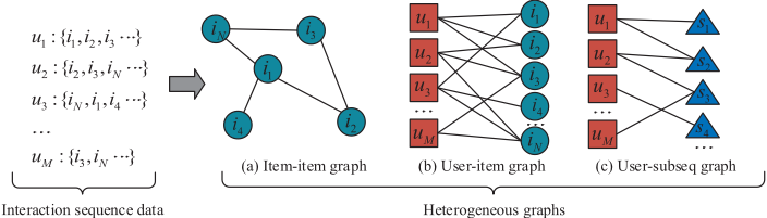
To solve these challenges, we first convert interaction sequences into three graphs including a user-item graph, an item-item graph, and a user-subseq graph to indicate the user preference over items, item dependency, and user similarity, respectively. In the graphs, neighbors are selected according to paths between vertices (path type and distance). Next, we propose a graph convolutional network named PGCN to learn the three kinds of information with the graphs and produce shared representations for users and items. The traditional convolution operation can only be applied on gridstructured input. But the graphs are in non-Euclidean domains and the convolution cannot handle the varied number of neighbors [Hechtlinger et al., 2017]. To address this issue, we design a neighbor pooling operation to cluster neighbors according to the path type and distance. For each target vertex, the pooling operation produces a fixed number of virtual vertices by aggregating features of its neighbors with attention mechanism. We perform a convolution operation on the virtual vertices and generate new latent vectors for each vertex (users or items). Then, our neural network outputs shared representations for users and items in heterogenous graphs. At last, the recommendation problem is formulated as an edge prediction task based on the representations.
In summary, our main contributions are as follows.
- We design three heterogeneous graphs for mining user preference, item dependency and user similarity information contained by interaction sequences for recommendation tasks.
- We propose a graph convolutional network, PGCN, to learn shared representations for users and items with the heterogeneous graphs. We offer a novel pooling operation to deal with a varied number of neighbors and design a graph convolution operation for aggregating features of neighbors and retaining the locality in graphs.
- Our approach outperforms several state-of-the-art methods in terms of hit ratio and NDCG on two real-world datasets. The experiments also prove that the heterogeneous graphs are effective for improving the recommendation performance.
2 Preliminary
2.1 Learning from Sequence Data
We first present several fundamental definitions.
Definition 1 (Interaction Sequence) For each user, his/her interaction records (i.e., < user, item, time >) can be sorted by timestamps and form sequences as shown in Figure 1.
Definition 2 (N-item subsequence) An n-item subsequence is a contiguous sequence of n items from a given interaction sequence of a user. For example, a user has a shopping sequence {pen, pencil, eraser}. Its 2-item subsequences are "pen, pencil" and "pencil, eraser". We use subsequences to denote all n-item subsequences.
We convert interaction sequences into following three graphs (Figure 1).
Definition 3 (User-item Interaction Graph) The user-item interaction graph GR = (V U ∪ V I ,ER) records interactions between users and items, where V U and V I denote sets of users and items, respectively, and |V U | = M, |V I | = N. ER ⊆ V U × V I is a set of edges. The weight of edge eu,i denotes the number of interactions between u and i.
Definition 4 (Item-itemGraph) The item-item graph, i.e., GI = (V I ,EI ), is designed to retain the dependency between items. The V I is the set of items. The weight of edge ei,j in EI ⊆ V I ×V I is the number of co-occurrence of item i and j (two adjacent items) in interaction sequences.
Definition 5 (User-subseq Graph) The user-subseq graph GU = (V U ∪ V G, EU ) is utilized to record interactions between users and subsequences and indicates user similarity on behaviors. V G is the set of n-item subsequences and EU ⊆ V U × V G is the set of edges in GU .
At last, we use G to denote the three graphs, i.e., G = GR ∪ GI ∪ GU . The three graphs can also be represented by adjacency matrices, i.e., AR ∈ R(M+N)×(M+N) , AI ∈ RN×N , AU ∈ R(M+O)×(M+O) . The elements in adjacency matrices record weights of edges in the corresponding graphs.
If there exists a path from vertex i to vertex j in a graph, we define the path type T(i, j) with the types of i and j. The number of edges in the path is defined as distance D(i, j) between the two vertices. For example, a path user1 → item1 → user3 in graph GR, its path type will be u-u (user to user) and distance will be 2.
| Distance=1 | Distance=2 | |||||
|---|---|---|---|---|---|---|
| Graphs | GI | GR | GU | GI | GR | GU |
| User | / | u- i | u- s | / | u-u | u-u |
| Item | i - i | i -u | / | i - i | i - i | / |
| Subseq | / | / | s -u | / | / | s - g |
Definition 6 (Neighbors) Neighbors of one vertex in heterogeneous graphs are chosen by two factors, i.e., path type and distance. We define neighbors of a vertex i as Nlt(i) = {j|D(i, j) = l, T(i, j) = t} where l is distance and t is path type. In addition, we define each vertex as its neighbor with distance equal to 0, i.e., N0,T(i)(i) = {i}. Neighbors of each kind of vertex are shown in Table 1.
2.2 Recommendation ProblemFormulation
In our work, interactions between users and items are represented by edges between vertices in graphs. The edges reflect users' preference on items. Therefore, the recommendation problem can be cast as an edge prediction task. More precisely, given the heterogeneous graphs G, we aim to predict the probability of existence of edge eu,i between vertex u and i, i.e., p(eu,i|G).
3 Learning Shared Vertex Representations
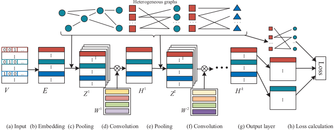
In this section, we propose a new graph convolutional neural network, Path conditioned Graph Convolutional Network (PGCN) as shown in Figure 2. In our approach, we represent vertex features and adjacency information with a matrix and heterogeneous graphs, respectively. In what follows, we introduce details of our approach layer by layer.
3.1 Input and Embedding Layer
As shown in Figure 2(a), each vertex (including users, items and n-item subsequences) is denoted by a one-hot vector vi indicating its ID. It should be noticed that properties or contents of vertices can also be concatenated with one-hot vectors to alleviate the data sparsity problem. As we aim to study the effect of convolution on a graph with information of neighbors, only one-hot vectors are employed for simplicity. We use matrix V ∈ Rd0×d0 (d0 = M + N + O) to store one-hot vectors of all vertices.
The one-hot vectors are transformed into embeddings of low dimensions with H0 = V E and E ∈ Rd0×d1 . The embedding of vertex i is denoted by h0i . The three graphs share embeddings and representations of users and items.
3.2 Neighbor Pooling
Now, we need to define a convolution operation to reserve the local connectivity of graphs. The traditional convolution operation cannot handle the varying number of neighbors for each vertex. However, another widely-used operation, i.e., pooling, can solve the problem. We employ the pooling operation to aggregate features of neighbors and produce a fixed number of virtual vertices. In previous research, pooling layers usually come after convolution layers. But the two operations are actually independent of each other. We can conduct a pooling operation before a convolution layer.
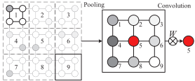
In Figure 3(a), the pooling operation is performed on 9 regions of an image with four nodes (pixels) in each of them. The regions are constructed with nodes according to their direction and distance to region 5. After pooling, a convolution operation is performed to produce the representation for node 5. Similarly, in graphs, we select neighbors by path type and distance to target vertices, i.e., Nlt(i), which is shown as Figure 3(b).
We introduce the processing details of neighbor pooling. First, neighbors are clustered by the path type and distance to a target vertex. Then, for each cluster, a neighbor pooling is performed and produces a virtual vertex. The equation for pooling is as below.
where Nlt(i) is the set of neighbors with distance l and path type t for vertex i. hk-1 j is the representation of vertex j in layer k - 1. αij is the weight for determining the importance of j for i. zi lt denotes one virtual vertex aggregated with neighbors Nlt of vertex i.
We provide two ways to calculate the weight αij , i.e., with transition probability or attention. We take the graph GR as an example. For GR, we have the adjacency matrix AR and define D as a diagonal matrix where Dii = ∑j ARij . Then the transition matrix for one hop can be obtained by S(1) = D-1AR. Based on the transition matrix S(1) , we can obtain a transition matrix for two hops with A′ = S(1)S(1) . We set
(a) Pooling and convolution on an image
Neighbor pooling Convolution
W
Users
Item
Items
(b) Pooling and convolution on a graph
Figure 3: Illustration of pooling and convolution operations (dashed line box) on an image or a graph. Ws are weights for convolution.
A′ii = 0 to remove the transition to the vertex itself. The matrix is normalized with S(2) = E-1A′ and E is a diagonal matrix where Eii = ∑j A′ij . We set αij to S(1) ij and S(2) ij for neighbors with distance equal to 1 and 2, respectively.
The weight αij can also be computed with the attention mechanism according to the following equation [Velickovic et al., 2017; He et al., 2018].
where f(·) is a fully connected neural network with two hidden layers.
We use term "PGCN-C" and "PGCN-A" to denote our approaches that use constant transition probability and attention mechanism, respectively.
3.3 Convolution
Convolution is conducted on the virtual vertices and generates new representations of vertices:
where zi lt is the feature vector of a virtual vertex with distance l and path type t for vertex i. L determines the size of filters, i.e., how many neighbors are considered. For example, if L = 1, neighbors within 1 hops will be utilized. In this paper, we only consider neighbors within 2 hops. W k lt ∈ Rdk×dk-1 and bklt ∈ Rdk are weights and bias for convolutional filters in layer k. All vertices in graphs share parameters W k lt and bklt for the same kinds of virtual vertices. g(·) is an activation function.
With several neighbor pooling and convolution layers, we can output a representation hi for each vertex.
3.4 Model Training
With the representations of users and items, we can compute the probability of the existence of each edge between users and items with ˆ p(eu,i|G) = σ(hu T hi). hu and hi are representations of user u and item i, respectively. The interaction function (inner product) between hu and hi can also be replaced by a fully connected neural network [He et al., 2017]. For the space limitation, we leave this to be studied in the future. σ is the sigmoid function. ˆ p(eu,i|G), ˆ pu,i for short, denotes the predicted probability of existence of edge eu,i. If a user has interacted with an item, the ground truth is set to 1, i.e., pu,i = 1. Otherwise, pu,i = 0. The loss for optimization can be defined with a cross-entropy function.
where Y = Y + ∪ Y -. Y + denotes the set of existing edges and Y - is a set of unobserved interactions between users and items. Given one interaction (u, i), negative instances (u, j) are sampled from items that user u has not interacted with. ω(θ) is the regularization term and λ is the weight of it.
4 Experiments
In the experiments, we aim to answer the following three questions.
RQ1: Do our approaches outperform other methods?
RQ2: Do the heterogeneous graphs provide valuable information beyond the user preference on items?
RQ3: How do hyper-parameters affect the performance?
4.1 Experimental Settings
| Dataset | # user | # item | # interaction |
|---|---|---|---|
| MovieLens | 943 | 1,682 | 100,000 |
| Retailrocket | 1,407,580 | 417,053 | 2,664,312 |
Datasets. In the experiments, we utilize two publicly available datasets including MovieLens-100K 1 and Retailrocket 2 . Their statistic information is summarized in Table 2. Their descriptions are as follows:
- MovieLens dataset collected ratings of movies (1-5 star) rated by users. We treated ratings as weights of edges between users and items in the user-item graph.
- Retailrocket dataset recorded user interactions including clicks, adding to carts, and transactions with items on a real-world e-commerce website. We filtered out users interacting with less than 10 items and items having less than 30 users to alleviate the sparsity problem.
Evaluation protocols. We adopt the leave-one-out evaluation method which is widely used in many works [He et al., 2017; He et al., 2018]. We compute average Hit Ratio (HR) [Deshpande and Karypis, 2004] and Normalized Discounted Cumulative Gain (NDCG) [He et al., 2017] by ranking 100 items (one selected testing instance and 99 sampled negative instances) for each user with predicted preference scores.
1 https://grouplens.org/datasets/movielens/
2 https://www.kaggle.com/retailrocket/ecommerce-dataset
| K=2 | K=6 | K=10 | ||||||||||
|---|---|---|---|---|---|---|---|---|---|---|---|---|
| MovieLens | Retailrocket | MovieLens | Retailrocket | MovieLens | Retailrocket | |||||||
| Methods | HR | NDCG | HR | NDCG | HR | NDCG | HR | NDCG | HR | NDCG | HR | NDCG |
| POP | 16.12 | 13.54 | 13.32 | 11.41 | 32.77 | 20.59 | 27.44 | 17.40 | 41.68 | 23.35 | 36.81 | 20.32 |
| BPR | 24.74 | 21.89 | 42.59 | 38.21 | 49.28 | 31.87 | 58.38 | 44.25 | 64.06 | 36.25 | 65.68 | 47.44 |
| FISM | 25.99 | 22.81 | 43.79 | 39.05 | 51.33 | 33.65 | 59.40 | 46.47 | 65.53 | 37.95 | 66.71 | 48.80 |
| SMF | 24.93 | 21.88 | 43.59 | 38.44 | 49.57 | 31.85 | 59.43 | 45.83 | 65.66 | 36.91 | 67.11 | 48.24 |
| sRMGCN | 26.36 | 23.12 | 44.78 | 38.73 | 49.65 | 32.66 | 59.53 | 46.32 | 66.47 | 37.93 | 67.77 | 48.96 |
| NAIS | 26.95 | 23.73 | 47.75 | 39.44 | 52.58 | 34.30 | 61.27 | 48.27 | 66.06 | 38.53 | 68.23 | 50.68 |
| PGCN-C | 29.71 | 25.14 | 46.93 | 43.48 | 53.59 | 35.35 | 64.88 | 49.36 | 67.99 | 39.86 | 72.62 | 51.52 |
| PGCN-A | 29.30 | 24.96 | 49.24 | 44.39 | 54.15 | 35.62 | 66.89 | 51.89 | 67.79 | 39.57 | 73.33 | 54.00 |
Baselines. We compare our approaches, PGCN-C and PGCN-A, with following recommendation methods.
- POP. This method ranks items by popularity [Koren and Bell, 2015].
- BPR. It adopts a pair-wise ranking loss function for MF models [Rendle et al., 2009].
- FISM. This method takes advantage of features of items that a user has interacted with to obtain better representations for users [Kabbur et al., 2013].
- SMF. Item embeddings are learned with a song2vec model and are used to compute item similarity as constraints in MF models [Cheng et al., 2017].
- sRMGCNN. It is a multi-graph convolutional neural network imposing smoothness priors on graphs [Monti et al., 2017].
- NAIS. NAIS adopts attention mechanism to aggregate features of items to represent users' profile [He et al., 2018].
Settings. We implemented our approaches using TensorFlow. To reduce the complexity, we only considered neighbors within two hops and selected at most 100 neighbors for each type. Only 2-item subsequences were utilized in graph GU . We chose the LeakyReLU activation function and utilized two pooling and convolution layers. We adopted the Adam optimizer to minimize our loss function and set the learning rate to 0.001. We chose the l2 regularization and the weight of it was set to 10-4 . The batch size was 512. To prepare the training dataset, we sampled four negative instances for each positive one. FISM and NAIS took all items that a user had interacted with as neighbors of him/her. sRMGCNN had three LSTM layers. For NAIS, the smoothing exponent was β = 0.5.
4.2 Experimental Results
Performance comparison (RQ1). Table 3 shows the performance of HR@K and NDCG@K with respect to the number of recommended items (i.e., K). For all methods, the size of latent vectors is set to 64. First, we can see that our approaches (PGCN-C and PGCN-A) achieve the best performance on the two datasets in terms of HR and NDCG. PGCNA achieves a relative improvement of 4.7% and 6.8% over NAIS in terms of HR on MovieLens and Retailrocket, respectively. We also find that PGCN-A seems to have better performance on Retailrocket dataset than PGCN-C and the situation is contrary on MovieLens. This may be because the MovieLens dataset is small and PGCN-A which is more complex than PGCN-C may have overfitting problem on it. Among all baselines, NAIS utilizes attention mechanism to aggregate features of neighbors (items) to represent users' profile and performs the best. FISM also uses this kind of information. But it treats all items equally and its performance is a little poorer than NAIS. sRMGCN uses spectral graph convolution to retain the locality of user-item graph and performs better than other baselines.
Effect of heterogeneous graphs (RQ2). To demonstrate the effectiveness of the heterogeneous graphs, we compare results of our approaches leveraging one or two kinds of graphs. As shown in Table 4, PGCN-C can achieve the best performance with all the three kinds of graphs (i.e., GR, GI , and GU ) on both datasets. PGCN-A has the best performance using all graphs on Retailrocket dataset. The two approaches both have a better performance by adding graph GI (indicating item dependency) or graph GU (indicating user similarity) than approaches with only graph GR on both datasets. Similar to Table 3, we can see that the performance improvement of adding GI and GU in Retailrocket is larger than that in MovieLens. This is because users may have many interactions with an item (buying one kind of item many times) and interaction sequences contain richer item dependency information and user similarity on behaviors in Retailrocket.
| Graphs | GR | GR+GI | GR+GU | G | |
|---|---|---|---|---|---|
| MovieLens | |||||
| PGCN-C | HR | 66.06 | 66.48 | 67.12 | 67.97 |
| NDCG | 38.13 | 38.62 | 38.75 | 39.42 | |
| HR | 67.02 | 67.76 | 68.39 | 67.76 | |
| PGCN-A NDCG | 38.68 | 39.22 | 39.75 | 39.57 | |
| Retail | |||||
| PGCN-C | HR | 69.00 | 71.35 | 69.60 | 72.51 |
| NDCG | 49.36 | 50.58 | 49.96 | 51.52 | |
| HR | 68.83 | 70.58 | 69.80 | 73.33 | |
| PGCN-A NDCG | 50.15 | 52.21 | 52.02 | 54.02 | |
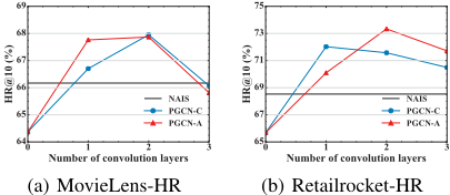
Effect of the number of convolution layers (RQ3). As PGCN is a neural network based method, a problem worth studying is that how many neural layers are appropriate for the recommendation tasks. We evaluate our approaches by varying the number of neural layers (a neighbor pooling and a convolution layer are as one neural layer). Experimental results are shown in Figure 4. For the space limitation, we only show the performance of HR@10. When the number of convolution layer is 0, our approaches become traditional matrix factorization methods. From the figure, we can see that our approaches with convolution layers are much better than that without convolution layers on both datasets. As the number of layers grows, the performance grows. When the number of layers is 3, the performance drops. We think our approaches may have overfitting problem when the number is 3.
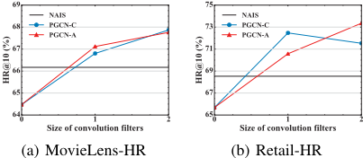
Effect of the filter size (RQ3). The size of convolution filters (i.e., L) can also affect the performance of our approaches. With larger convolution filters, our approaches can aggregate features of more neighbors. We show results of our approaches with different sizes of convolution filters in Figure 5. When the size is bigger, the number of neighbors grows exponentially. Therefore, we only evaluate the size of 1 and 2. Our approaches become traditional MF methods when the size of filters is 0. We can see that with convolution, our approaches achieve better performance on both datasets. The performance becomes better when the size of filters grows. For PGCN-C, the performance drops a little on Retailrocket dataset when the size of filters is 2. We think convolution operation may bring noise when the filter size is too large.
5 RelatedWork
Matrix Factorization (MF) as one of the most popular recommendation technics is used to model users' preference based on explicit ratings [Koren et al., 2009] or implicit feedbacks [Hu et al., 2008], and is enhanced with advanced pair-wise loss function [Rendle et al., 2009] and interaction function [He et al., 2017]. Based on interaction data, features of neighbors defined by the interactions are also used for improving the performance [Kabbur et al., 2013; He et al., 2018]. Besides the direct interaction, dependency among items in interaction sequences is also modeled by various approaches including Markov Chain [Feng et al., 2015], tensor decomposition [Cheng et al., 2013; Li et al., 2017], and RNN [Song et al., 2016; Yoo et al., 2017].
Besides the above technics, convolutional neural network is another effective method to take advantages of features of neighbors which has been proven in various domains including computer vision and natural language processing [LeCun et al., 2015; Hinton et al., 2012]. To deal with a varied number of neighbors in arbitrary graphs, researchers proposed to design new convolutions in spectral domain [Bruna et al., 2013; Henaff et al., 2015] or spatial domain [Bruna et al., 2013]. Compared to spectral methods, spatial convolution approaches are more flexible and design spatial convolution kernels by sharing weights based on the distance between two vertices [Atwood and Towsley, 2016] or performing random walks on graphs [Hechtlinger et al., 2017]. Nguyen [2018] and Simonovsky [2017] designed convolution filters whose weights were conditioned on edge types. The spectral and spatial convolutional networks have been both applied on the user-item interaction graph for recommendation [Monti et al., 2017; Berg et al., 2017]. But they only use direct interactions between users and items and omit item dependency and user similarity information.
6 Conclusion
In this paper, we converted interaction sequences to three heterogeneous graphs and proposed to mine three kinds of information for item recommendation. We aggregated features of neighbors defined with paths in the graphs, and proposed a convolutional network, PGCN, which has novel neighbor pooling and convolution operations for learning shared representations of users and items in the heterogeneous graphs. The operations can retain the locality of graphs and deal with the varied number of neighbors. Experiments on two datasets showed that our approach outperformed other methods. Besides recommendation, PGCN is a general method and can be applied in other domains.
Acknowledgements
This research is supported in part by NSFC (No. 61772341, 61472254, 61772338) and STSCM (No. 18511103002). This work is also supported by the Program for Changjiang Young Scholars in University of China, the Program for China Top Young Talents, the Program for Shanghai Top Young Talents, Shanghai Engineering Research Center of Digital Education Equipment, and SJTU Global Strategic Partnership Fund (2019 SJTU-HKUST). Yanyan Shen is supported by NSFC No. 61602297.
@inproceedings{ijcai2019p642,
  title     = {Learning Shared Vertex Representation in Heterogeneous Graphs with Convolutional Networks for Recommendation},
  author    = {Xu, Yanan and Zhu, Yanmin and Shen, Yanyan and Yu, Jiadi},
  booktitle = {Proceedings of the Twenty-Eighth International Joint Conference on
               Artificial Intelligence, {IJCAI-19}},
  publisher = {International Joint Conferences on Artificial Intelligence Organization},
  editor    = {Sarit Kraus},
  pages     = {4620--4626},
  year      = {2019},
  month     = {8},
  note      = {Main track},
  doi       = {10.24963/ijcai.2019/642},
  url       = {https://doi.org/10.24963/ijcai.2019/642},
}
TY - CPAPER TI - Learning Shared Vertex Representation in Heterogeneous Graphs with Convolutional Networks for Recommendation AU - Xu, Yanan AU - Zhu, Yanmin AU - Shen, Yanyan AU - Yu, Jiadi T2 - Proceedings of the Twenty-Eighth International Joint Conference on Artificial Intelligence, IJCAI-19 PB - International Joint Conferences on Artificial Intelligence Organization PY - 2019 SP - 4620 EP - 4626 DO - 10.24963/ijcai.2019/642 UR - https://doi.org/10.24963/ijcai.2019/642 ER -Copied
Machine-readable versions of this paper, for tools and AI agents:





