
Bayesian Inference of Linear Temporal Logic Specifications for Contrastive Explanations
Proceedings of the Twenty-Eighth International Joint Conference on Artificial Intelligence. Main track. Pages 5591-5598.
https://doi.org/10.24963/ijcai.2019/776
Keywords
- Planning and Scheduling: Search in Planning and Scheduling
- Planning and Scheduling: Activity and Plan Recognition
- Humans and AI: Human-AI Collaboration
Abstract
Temporal logics are useful for providing concise descriptions of system behavior, and have been successfully used as a language for goal definitions in task planning. Prior works on inferring temporal logic specifications have focused on "summarizing" the input dataset - i.e., finding specifications that are satisfied by all plan traces belonging to the given set. In this paper, we examine the problem of inferring specifications that describe temporal differences between two sets of plan traces. We formalize the concept of providing such contrastive explanations, then present BayesLTL - a Bayesian probabilistic model for inferring contrastive explanations as linear temporal logic (LTL) specifications. We demonstrate the robustness and scalability of our model for inferring accurate specifications from noisy data and across various benchmark planning domains.
- [Anastasiou, 2006] Alexander B Anastasiou. Modeling ur- ban warfare: Joint semi-automated forces in urban resolve. Technical report, Air Force Inst. of Tech, 2006.
- [Blei et al., 2003] David M Blei, Andrew Y Ng, and Michael I Jordan. Latent dirichlet allocation. JMLR, 3:993-1022, 2003.
- [Borgo et al., 2018] Rita Borgo, Michael Cashmore, and Daniele Magazzeni. Towards providing explanations for AI planner decisions. IJCAI Workshop on XAI, 2018.
- [Camacho and McIlraith, 2019] Alberto Camacho and Sheila A. McIlraith. Learning interpretable models expressed in linear temporal logic. In ICAPS, 2019.
- [Camacho et al., 2017] Alberto Camacho, Eleni Triantafil- lou, Christian J. Muise, Jorge A. Baier, and Sheila A. McIlraith. Non-deterministic planning with temporally ex- tended goals: LTL over finite and infinite traces. In AAAI, pages 3716-3724, 2017.
- [Chakraborti et al., 2017] Tathagata Chakraborti, Sarath Sreedharan, Yu Zhang, and Subbarao Kambhampati. Plan explanations as model reconciliation: Moving beyond explanation as soliloquy. In IJCAI, page 156-163, 2017. IJCAI
- [Chib and Greenberg, 1995] Siddhartha Chib and Edward Greenberg. Understanding the metropolis-hastings algo- rithm. The American Statistician, 49(4):327-335, 1995.
- [De Giacomo and Vardi, 2013] Giuseppe De Giacomo and Moshe Y Vardi. Linear temporal logic and linear dynamic logic on finite traces. In IJCAI, 2013.
- [Dzifcak et al., 2009] Juraj Dzifcak, Matthias Scheutz, Chitta Baral, and Paul Schermerhorn. What to do and how to do it: Translating natural language directives into temporal and dynamic logic representation for goal management and action execution. In ICRA, 2009.
- [Elzein, 2018] Nadine Elzein. The demand for contrastive explanations. Philosophical Studies, pages 1-15, 2018.
- [Göbelbecker et al., 2010] Moritz Göbelbecker, Thomas Keller, Patrick Eyerich, Michael Brenner, and Bernhard Nebel. Coming up with good excuses: What to do when no plan can be found. In ICAPS, 2010.
- [Hoffmann et al., 2004] Jörg Hoffmann, Julie Porteous, and Laura Sebastia. Ordered landmarks in planning. JAIR, 22:215-278, 2004.
- [Kasenberg and Scheutz, 2017] Daniel Kasenberg and Matthias Scheutz. Interpretable apprenticeship learning with temporal logic specifications. In CDC, 2017.
- [Katz et al., 2018] Michael Katz, Shirin Sohrabi, Octavian Udrea, and Dominik Winterer. A novel iterative approach to top-k planning. In ICAPS, 2018.
- [Kim et al., 2017] Joseph Kim, Christopher J Banks, and Julie A Shah. Collaborative planning with encoding of users' high-level strategies. In AAAI, pages 955-962, 2017.
- [Kong et al., 2017] Zhaodan Kong, Austin Jones, and Calin Belta. Temporal logics for learning and detection of anomalous behavior. IEEE Trans. on Automatic Control, 62(3):1210-1222, 2017.
- [Lemieux et al., 2015] Caroline Lemieux, Dennis Park, and Ivan Beschastnikh. General LTL specification mining (t). In Proc. ASE, pages 81-92, 2015.
- [Lombrozo, 2006] Tania Lombrozo. The structure and func- tion of explanations. Trends in Cognitive Sciences, 10(10):464-470, 2006.
- [Long and Fox, 2003] Derek Long and Maria Fox. The 3rd International Planning Competition: results and analysis. JAIR, 20:1-59, 2003.
- [Magnaguagno et al., 2017] Maurıcio C Magnaguagno, Ra- mon Fraga Pereira, Martin D Móre, and Felipe Meneguzzi. Web planner: A tool to develop classical planning domains and visualize heuristic state-space search. In UISP, 2017.
- [Neider and Gavran, 2018] Daniel Neider and Ivan Gavran. Learning linear temporal properties. In FMCAD, 2018.
- [Nguyen et al., 2012] Tuan Anh Nguyen, Minh Do, Al- fonso Emilio Gerevini, Ivan Serina, Biplav Srivastava, and Subbarao Kambhampati. Generating diverse plans to han- dle unknown and partially known user preferences. Artifi- cial Intelligence, 190:1-31, 2012.
- [Pnueli, 1977] Amir Pnueli. The temporal logic of programs. In Annual Symposium on Foundations of Computer Sci- ence, pages 46-57, 1977.
- [Ramırez and Geffner, 2010] Miquel Ramırez and Hector Geffner. Probabilistic plan recognition using off-the-shelf classical planners. In AAAI, 2010.
- [Seegebarth et al., 2012] Bastian Seegebarth, Felix Müller, Bernd Schattenberg, and Susanne Biundo. Making hy- brid plans more clear to human users-a formal approach for generating sound explanations. In ICAPS, 2012.
- [Shah et al., 2018] Ankit Shah, Pritish Kamath, Shen Li, and Julie Shah. Bayesian inference of temporal task specifica- tions from demonstrations. In NIPS, 2018.
- [Sohrabi et al., 2016] Shirin Sohrabi, Anton V Riabov, and Octavian Udrea. Plan recognition as planning revisited. In IJCAI, pages 3258-3264, 2016.
- [Veloso and Blythe, 1994] Manuela M Veloso and Jim Blythe. Linkability: Examining causal link commitments in partial-order planning. In AIPS, 1994.
- [Yang et al., 2006] Jinlin Yang, David Evans, Deepali Bhardwaj, Thirumalesh Bhat, and Manuvir Das. Perra- cotta: mining temporal API rules from imperfect traces. In ICSE, pages 282-291, 2006.
- [Yoo and Belta, 2017] Chanyeol Yoo and Calin Belta. Rich time series classification using temporal logic. In RSS, 2017.
- [Zhang et al., 2017] Yu Zhang, Sarath Sreedharan, Anagha Kulkarni, Tathagata Chakraborti, Hankz Hankui Zhuo, and Subbarao Kambhampati. Plan explicability and pre- dictability for robot task planning. In ICRA, 2017.
References were extracted automatically from the PDF and may contain errors.
Full text extracted automatically from the PDF; figures, tables and equations may differ. The PDF is the version of record.
1 Introduction
In this paper, we examine the problem of generating explanations for how two sets of plans differ in behavior. We focus on generating such contrastive explanations by discovering logical specifications that are satisfied (entailed) by one set of plans, but not the other. Prior works on plan explanations include those related to plan recognition for inferring latent goals through observations [Ramırez and Geffner, 2010; Sohrabi et al., 2016], works on system diagnosis and excuse generation in order to explain plan failures [Göbelbecker et al., 2010], and those focused on synthesizing "explicable" plans - i.e., plans that are self-explanatory with respect to a human's mental model [Zhang et al., 2017]. The aforementioned works, however, only involve the explanation or generation of a single plan; we instead focus on explaining differences between multiple plans, which can be helpful in various applications, such as the analysis of competing systems, classification of user-groups, and detection of anomalies.
A specification language should be used in order to achieve clear and effective plan explanations. Prior works have considered surface-level metrics such as plan costs and action (or causal link) similarity measures to describe plan differences
[Nguyen et al., 2012; Borgo et al., 2018]. In this work, we utilize Linear Temporal Logic (LTL) [Pnueli, 1977], which is an expressive language for capturing temporal relations across state variables. Planning is sequential, so temporal properties can offer greater expressivity and explanatory power for describing the high-level behavior of plans than static facts. We use plans' individual satisfaction (or dissatisfaction) of LTL specifications in order to describe their differences.
LTL specifications have been widely used in both industrial systems and planning algorithms to compactly describe temporal behavior [Yang et al., 2006]. Their declarative and compositional structure allows a straightforward translation to natural language, and inversely, LTL can be derived from natural language directives [Dzifcak et al., 2009]. Experiments also suggest that LTL formulas serve as natural patterns when encoding high-level human strategies as planning constraints [Kim et al., 2017].
Although a suite of LTL miners have been developed for software engineering and verification purposes [Yang et al., 2006; Lemieux et al., 2015; Shah et al., 2018], they primarily focus on mining properties that summarize the overall behavior on a single set of traces. Recently, SAT-based methods have been introduced to construct a LTL specification that asserts contrast between two sets of traces [Neider and Gavran, 2018; Camacho and McIlraith, 2019]. These exact learning algorithms, however, are designed to output a single minimallength formula, and are susceptible to failure when the input dataset contains imperfect traces. We examine a similar problem of mining contrastive explanations between two input sets, but adopt a probabilistic approach - we present BayesLTL, a Bayesian inference model that can quickly generate multiple explanations while demonstrating robustness to noisy input. This is important for real-world applications, where traces can contain noise not only from sensors and but from unintended user behavior (e.g., backtracking, misclicking on a page). BayesLTL permits scalability when searching in large hypothesis spaces and allows flexibility in incorporating various forms of prior knowledge and system designer preferences during search. We demonstrate the efficacy of our model for extracting multiple accurate explanations on noisy traces across various benchmark planning domains and for a simulated air combat mission.
2 RelatedWork
Plan explanations are becoming increasingly important as automated planners and humans collaborate. This first involves humans making sense of the planner's output, where prior work has focused on developing user-friendly interfaces that provide graphical visualizations to describe the causal links and temporal relations of plan steps [Seegebarth et al., 2012; Magnaguagno et al., 2017]. These systems, however, require an expert for interpretation and do not provide a direct explanation as to why the planner made certain decisions to realize the outputted plan.
Automatic generation of explanations has been studied in goal recognition settings, where the objective is to infer the latent goal state that best explains the incomplete sequence of observations [Ramırez and Geffner, 2010; Sohrabi et al., 2016]. Works on explicable planning emphasize the generation of plans that are deemed self-explanatory, defined in terms of optimizing plan costs for a human's mental model of the world [Zhang et al., 2017]. Mixed-initiative planners iteratively revise their plan generation based on user input (e.g. action modifications), indirectly promoting an understanding of differences across newly generated plans through continual user interaction [Borgo et al., 2018]. All aforementioned works deal with explainability with respect to a single planning problem specification, whereas our model deals with explaining differences in specifications governing two distinct sets of plans given as input.
Works on model reconciliation focus on producing explanations for planning models (i.e. preconditions and effects), instead of the realized plans [Chakraborti et al., 2017]. Explanations are specified in the form of model updates, iteratively bringing an incomplete model to a more complete model. The term, "contrastive explanation," is used in these works to identify the relevant differences between the input pair of models. Our work is similar in spirit but focuses on producing a specification of differences in the constraints satisfied among the realized plans. Our approach only requires sets of observed plan traces as input rather than environment models.
While model updates are an important modality for providing plan explanations, there are certain limitations. We note that an optimal plan generated with respect to a complete environment/world model is not always explicable or selfexplanatory. The space of optimal plans may be large, and the underlying preference or constraint that drives the generation of a particular plan may be difficult to pre-specify and incorporate within the planning model representation. We focus on explanations stemming directly from the realized plans themselves. Environment/world models (e.g. PDDL domain files) can be helpful in providing additional context, but are not necessary for our approach.
Our work leverages LTL as an explanation language. Temporal patterns can offer greater expressivity and explanatory power in describing why a set of plans occurred and how they differ, and may reveal hidden dynamics that cannot be captured by the use of surface-level metrics like plan costs or action similarities. LTL can represent temporally extended (i.e., non-Markovian) patterns like safety and reachability rules, and complex patterns across state variables.
Prior research into mining LTL specifications has focused on generating a "summary" explanation of the observed traces. Kasenberg and Scheutz [2017] explored mining globally persistent specifications from demonstrated action traces for a finite state Markov decision process. Lemieux et al. [2015] introduced Texada, a system for mining all possible instances of a given LTL template from an output log where each unique string is represented as a new proposition. Shah et al. [2018] proposed a template-based probabilistic model to infer task specifications given a set of demonstrations. However, all of these approaches focus on inferring a specification that all the observation traces satisfy.
For contrastive explanations, Neider and Gavran [2018] and Camacho and McIlraith [2019] presented SAT-based algorithms to infer a minimal-length LTL specification that delineates between the positive and negative sets of traces. Unlike existing LTL miners, these algorithms construct an arbitrary LTL specification without requiring predefined templates. However, they are designed to output only a single specification, 1 and can fail when the sets contain imperfect traces (i.e., if there exists no specification consistent with every single input trace.). We present a probabilistic model for the same problem and generate multiple contrastive explanations while offering robustness to noisy input.
Some works have proposed algorithms to infer contrastive explanations for continuous valued time-series data based on restricted signal temporal logic (STL) [Yoo and Belta, 2017; Kong et al., 2017]. However, the continuous space semantics of STL and a restricted subset of temporal operators make the grammar unsuitable for use with planning domain problems. To the best of our knowledge, our proposed model is the first probabilistic model to infer contrastive explanations for sets of traces in domains defined by PDDL.
3 Preliminaries
3.1 Linear Temporal Logic
Linear Temporal Logic (LTL) provides an expressive grammar for describing temporal behavior [Pnueli, 1977]. An LTL specification ϕ is constructed from a set of propositions V , the standard Boolean operators, and a set of temporal operators. Its truth value is determined with respect to a trace, π, which is an infinite or finite sequence of truth assignments for all propositions in V . The notation π, t |= ϕ indicates that ϕ holds at time t. The trace π satisfies ϕ (denoted by π |= ϕ) iff π, 0 |= ϕ. The minimal syntax for LTL can be described as follows:
where p is a proposition, and ϕ1 and ϕ2 are valid LTL specifications.
X reads as "next" where Xϕ evaluates as true at t if ϕ holds in the next time step t + 1. U reads as "until" where ϕ1Uϕ2 evaluates as true at time step t if ϕ1 is true at that time and going forward, until a time step is reached where ϕ2
1 In order to generate multiple explanations, the prior methods would require further queries, which involves iterating on the whole original algorithm.
| Template | nT | Formula | Meaning |
|---|---|---|---|
| ϕglobal | 1 | Gpi | pi is true throughout the entire trace. |
| ϕeventuality | 1 | Fpi | pi eventually occurs (may later become false). |
| ϕatmostonce | 1 | G(pi → (piWG¬pi)) | Only one contiguous interval exists where pi is true. |
| ϕstability | 1 | FGpi ∧ G(pi → (piWG¬pi)) | pi eventually occurs and stays true forever. |
| ϕuntil | 2 | piUpj | pi has to be true until pj eventually becomes true. |
| ϕresponse | 2 | G(pi →XFpj) | If pi occurs, pj eventually follows. |
| ϕprecedence | 2 | (pj ∧ ¬pi)R(¬pi) | If pi occurs, pj occurred in the past. |
becomes true. In addition to the minimal syntax, we also use higher-order temporal operators: F (eventually), G (global), W (weak until), and R (release). Fϕ holds true at t if ϕ holds for some time step ≥ t. Gϕ holds true at t if ϕ holds for all time steps ≥ t. ϕ1Wϕ2 is equivalent to ϕ1U(ϕ2 ∨ Gϕ1), where it does not enforce ϕ2 to occur. ϕ1Rϕ2 holds true at time step t if either there exists a time step t1 ≥ t such that ϕ2 holds true until t1 where both ϕ1 and ϕ2 hold true simultaneously, or no such t1 exists and ϕ2 holds true for all time steps ≥ t.
Interpretable sets of LTL templates have been defined and successfully integrated for a variety of software verification systems [Yang et al., 2006]. Some of the widely used templates are shown in Table 1.
3.2 Contrastive Explanation
According to Elzein [2018], a contrastive explanation describes "why event A occurred as opposed to some alternative event B." In our problem, events A and B represent two sets of plan traces. The form of why may be expressed in various ways [Lombrozo, 2006]; our choice is to define it according to the plans' satisfaction of a constraint. Then, formally:
Definition 3.1. A contrastive explanation is a constraint ϕ that it is satisfied by one set of plan traces (positive set, πA), but not by the other (negative set, πB).
The constraint ϕ can be seen as a behavior classifier trying to separate the provided positive and negative traces. Its performance measure corresponds to standard classification accuracy, computed by counting the number of traces in πA that satisfy ϕ and, conversely, the number of traces in πB where ϕ is unsatisfied. Formally, accuracy of ϕ is:
Accuracy is 1 for a perfect contrastive explanation, and approaches zero if both sets contains no valid trace with respect to ϕ (i.e., all traces in πA dissatisfy ϕ and all traces in πB satisfy ϕ).
4 Problem Statement and Approach
The input to the problem is a pair of sets of traces (πA, πB). Each πi ∈ π is a trace on the set of propositions V (we refer to V as the vocabulary). The output is a set of specifications, {ϕ}, where each ϕ achieves perfect or near-perfect contrastive explanation. We use LTL specifications for the choice of ϕ and utilize a set of interpretable LTL templates that are widely used in the development of software systems, such as those shown in Table 1.
4.1 Hypothesis Space
Our hypothesis space is restricted to a finite set of LTL templates. Once a LTL template T is selected, it is instantiated with a selection of nT propositions denoted by p ∈ V nT . The candidate formula ϕ is then composed as a conjunction of multiple instantiations of a template T based on a set of selections {p} ⊆ V nT . For example, an instantiation of T = "global" with p = [apple] is written as G(apple). If the selected subset of propositions is {p} = {[apple], [banana], [carrot]}, then ϕ = G(apple) ∧ G(banana) ∧G(carrot), asserting the global condition for all three propositions. Conjunctions can provide powerful semantics with the ability to capture a notion of quantification. Formally, our LTL specification is written as follows:
Note that the number of free propositions, nT , varies per LTL template. The number of possible specifications for a given LTL template T is 2|V |nT . Instead of extracting specifications narrowed down to a single template query, our hypothesis space Φ is set to include a number of predefined templates, T1, T2, ...Tk. With k representing the number of possible templates, the full hypothesis space of Φ grows with O(k · 2|V |nT ). Employing brute force enumeration to find {ϕ} that achieves the contrastive explanation criterion rapidly becomes intractable with increasing vocabulary size.
The graphical model shown in Figure 1 visually depicts the production rules of our hypothesis space. Note that we could have expressed the rules as a context-free grammar, but due to constraints such as the sharing of templates across conjuncts, it would have not resulted in a compact representation.
4.2 Bayesian Inference
We model specification learning as a Bayesian inference problem, building on the fundamental Bayes theorem:
Our goal is to infer ϕ∗ = argmaxΦP(ϕ|X). P(ϕ) represents the prior distribution over the hypothesis space, and P(X | ϕ) is the likelihood of observing the evidence X =
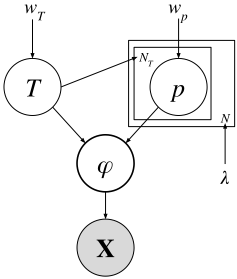
(πA, πB) given ϕ. We adopt a probabilistic generative modeling approach that has been used extensively in topic modeling [Blei et al., 2003]. Below, we describe each component of our generative model, depicted in Figure 1.
Prior Function
Our prior function serves as a preference module for the system designer. ϕ is generated by choosing a LTL template, T , the number of conjunctions, N, and then the proposition instantiations, p for each conjunct. The generative process for each of those components is as follows:
T is generated with respect to a categorical distribution with weights wT ∈ Rk over the k possible LTL templates. wT is a hyperparameter that the designer can set to assert preferences for mining certain types of templates over others (e.g., preferring templates with "global" operators than "until" operators).
The number of conjunctions, N = |{p}|, is generated using a geometric distribution with a decay rate of λ. Thus, the the probability of ϕ is reduced by λ for each addition of a conjunct, incentivizing low-complexity specifications defined in terms of having a fewer number of conjunctions (which also implies fewer total propositions). This promotes conciseness and prevents over-fitting to the input traces (i.e., to avoid restating the input as a long, convoluted LTL formula).
Similar to the method used for template selection, we use a separate categorical distribution for selecting propositions p for each conjunct in ϕ. Propositions are generated with respect to the probability weights, wp ∈ R|V | , defined for all p in V. The designer can likewise control wp to favor specifications instantiated with certain types of propositions over others. wp may be interpreted as the level of saliency of propositions for an application. (For example, propositions that are landmarks for planning problems [Hoffmann et al., 2004], or a part of the causal links set [Veloso and Blythe, 1994], may be deemed more important to express in plan explanations than other auxiliary state variables.) Several forms of variable importance, corresponding to the saliency of that importance in an explanation, may be applied to set wp. This opens the door to hypothesizing which propositions are most salient for a given domain, and generating explanations restricted to those propositions exclusively.
The full prior function, P(ϕ), is evaluated as follows:
The derivation follows from the definition that T, N, {p} completely describe ϕ (i.e. P(ϕ | T,N, {p}) = 1), and the assumption that the three probability distributions are independent of each other. P(T) and P(N) are calculated using categorical and geometric distributions outlined in Equations 5 and 6, respectively. P({p}) denotes the probability of the full set of proposition instantiations (over all conjuncts); it is calculated by the average categorical weight, wp, over all propositions. Formally:
For example, with {p} = {[a, b], [a, c], [b, c]}, and wa = 5/10, wb = 4/10, wc = 1/10, P({p}) = 20/10 6 = 1/3.
Likelihood Function
Our likelihood function is responsible for asserting contrast between the two input sets. P(X | ϕ) is the probability of observing the input sets of traces in the satisfying set πA and the non-satisfying set πB given the contrastive specification. The traces in πA and πB are generated by different solutions to the planning problem that satisfy the problem specification. As the problem specification is the only input needed to generate a set of plans, we assume that the individual traces are conditionally independent of each other, given the planning problem specification. With the conditional independence assumption, the likelihood can then be factored as follows:
LTL satisfaction checks are conducted over all traces belonging to sets πA and πB; P(πi|ϕ) is set equal to 1 - α if πi |= ϕ, and α otherwise. Conversely, P(πj|ϕ) is set equal to 1-β if πj ⊭ ϕ, and β otherwise. α and β permit non-zero probability to traces not adhering to the constrastive explanation criterion, thereby providing robustness to noisy traces and outliers. α and β may be set to different values to reflect the relative importance of the positive and negative sets.
In order to perform LTL satisfaction checks on a trace, we follow the method developed by Lemieux et al. [2015], in which ϕ is represented as a tree and each temporal operator is recursively evaluated according to its semantics. Since subtrees of two different ϕ may be identical, we memoize and re-use evaluation results to significantly speed up LTL satisfaction checks. We follow the semantics of LTL interpreted over finite traces [De Giacomo and Vardi, 2013].
Proposal Function
Exact inference methods to find maximum a posterior (MAP) estimates, {ϕ∗ }, are intractable. Thus we implement a Markov Chain Monte Carlo method, specifically the Metropolis-Hasting (MH) algorithm [Chib and Greenberg, 1995], to iteratively draw samples whose collection approximates the true posterior distribution. MH sampling requires a user-defined proposal function F(ϕ′ |ϕ) that samples a new candidate ϕ′ given the current ϕ. Our F behaves similar to an ϵ-greedy search, utilizing a drift kernel (i.e. a random walk) with a probability of 1 - ϵ or sampling from the prior distribution (i.e. a restart) with a probability of ϵ. The drift kernel operates by performing one of the following moves on the current candidate LTL ϕ:
- Remain within the current template T, add a new conjunct, and instantiate that conjunct with a randomly sampled p that is currently not in ϕ. The probability associated with this move, Qadd, is equal to 1/(|VnT | -N).
- Remain within the current template T and randomly remove one of the existing conjuncts. The probability associated with this move, Qremove, is equal to 1/N.
The selection between these two moves is conducted uniformly, though there is no issue with allowing the designer to weight one more likely than the other. Note that the drift kernel perturbs ϕ, but stays within the current template. ϕ transitions to a new template (probabilistically) when choosing to sample from the prior distribution, which has support over the full hypothesis space.
The probability distribution associated with F , denoted by Q(ϕ′ |ϕ), is then outlined as follows:
Our proposal function F fulfills the ergodicity condition of the Markov process (the transition from any ϕ to ϕ′ is aperiodic and occurs within a finite number of steps), thus asymptotically guarantees the sampling process from the true posterior distribution.
A new sample ϕ′ is accepted at every MH iteration with the following probability:
The set of accepted samples approximates the true posterior, and the MAP estimates (the output {ϕ∗ }) are determined from the relative frequencies of accepted samples.
Model Summary
Overall, the inductive biases of BayesLTL include 1) a bias towards having simpler explanations, 2) designer-controlled biases towards mining preferred templates and propositions, and 3) a search bias towards considering candidate specifications that are syntactically similar to the incumbent sample. These biases are all incorporated and jointly factored in a single Bayesian inference model.
5 Evaluations
5.1 Derivation of Evaluation Dataset
We evaluated the effectiveness of BayesLTL for inferring contrastive explanations from sets of traces generated from International Planning Competition (IPC) planning domains [Long and Fox, 2003]. The plan traces in πA were generated by first injecting the ground truth ϕground into the original PDDL domain/problem files, enforcing valid plans on the modified domain/problem files to satisfy ϕground. The LTL injection to create modified files was performed using the ltlfond2fond tool [Camacho et al., 2017]. Second, a state-ofthe-art top-k planner [Katz et al., 2018] was used to produce a set of distinct, valid plans and their accompanying state execution traces. (An alternative would have been to use a diverse planner [Nguyen et al., 2012], but the existing ones did not support the required expressivity of conditional effects in the modified planning files.)
Similarly, the above steps were repeated to generate execution traces for πB, wherein the negation of the ground truth specification, ¬ϕground, was injected to the planning files, and then a set of traces was collected. Such a setup guarantees the existence of contrastive explanation solutions on (πA, πB), which includes (but is not limited to) ϕground. We collected twenty traces for each set.
We evaluated our model using six different IPC benchmark domains, containing problems related to mission planning, vehicle routing, and resource allocation. For each of these domains, we tested three different problem instances of increasing vocabulary size, and on twenty randomly generated ϕground specifications for each problem instance.
5.2 Experiment Details
For each test case, ϕground was randomly generated using one of the seven LTL templates listed in Table 1; thus the hypothesis space Φ was set to include all possible specifications over the predefined templates. The categorical distribution weights, wT and wp, were set to be uniform. Other hyperparameters were set as follows: α = β = 0.01, to put equal importance of positive and negative sets, λ = 0.7 to penalize ϕ for every additional conjunct, and ϵ = 0.2 to apply ϵ-greedy search in the the proposal function. We ran the MH sampler with numMH = 2, 000 iterations with the first 300 used as a burn-in period. Our experimental results were found to be robust to the various settings of these hyperparameters (evaluated by a grid search).
5.3 Model Comparisons
We evaluated BayesLTL against the SAT-based miner 2 developed by Neider and Gavran [2018], the state-of-the-art for extracting contrastive LTL specifications. We also evaluated our model against brute force enumeration, a common approach employed by existing LTL miners for summarization [Yang et al., 2006; Lemieux et al., 2015]. Because enumerating through full space of Φ would result in a time out, we tested delimited enumeration with only a random subset of brute force samples. This baseline selects a random subset of size numbrute from Φ. Then, a function proportional to the posterior distribution (numerator in Equation 4) is evaluated for each of the samples to determine {ϕ∗ }. numbrute was set equal to numMH to enable a fair baseline in terms of having the same amount of allotted computation. All experiments were conducted on Debian machines with Intel Xeon E3-1200 CPUs at 1.8 GHz using up to 4 GB of RAM.
2 https://github.com/gergia/samples2LTL (commit: 69f692a).
| Domain | |V | | BayesLTL | Enumeration | Neider &Gavran | |||
|---|---|---|---|---|---|---|---|
| M | Acc | M | Acc | M | TimeOut | ||
| blocks- world | 16 | 3.1 | 0.97 | 0.9 | 0.96 | 1 | 10 / 20 |
| 25 | 8.1 | 1.00 | 0.8 | 0.95 | 1 | 10 / 20 | |
| 55 | 30.2 | 0.99 | 0.7 | 0.83 | 0 | 20 / 20 | |
| storage | 11 | 4.4 | 0.94 | 1.7 | 0.97 | 1 | 16 / 20 |
| 20 | 11.5 | 0.97 | 1.0 | 0.94 | 1 | 14 / 20 | |
| 42 | 31.5 | 0.98 | 0.9 | 0.93 | 1 | 11 / 20 | |
| satellite | 17 | 22.3 | 1.00 | 3.7 | 0.97 | 1 | 6 / 20 |
| 37 | 28.0 | 0.98 | 0.9 | 0.85 | 1 | 8 / 20 | |
| 50 | 84.6 | 0.97 | 1.0 | 0.94 | 1 | 8 / 20 | |
| zeno- travel | 18 | 3.7 | 0.99 | 2.1 | 0.99 | 1 | 8 / 20 |
| 22 | 21.0 | 1.00 | 1.7 | 0.99 | 1 | 8 / 20 | |
| 40 | 78.6 | 0.99 | 1.5 | 0.99 | 1 | 3 / 20 | |
| TPP | 14 | 7.5 | 1.00 | 1.1 | 0.95 | 0 | 20 / 20 |
| 18 | 9.7 | 1.00 | 0.8 | 0.95 | 0 | 20 / 20 | |
| 36 | 114.5 | 0.99 | 2.3 | 0.96 | 1 | 14 / 20 | |
| rovers | 20 | 24.5 | 1.00 | 2.3 | 0.99 | 1 | 5 / 20 |
| 22 | 28.3 | 1.00 | 2.3 | 0.99 | 1 | 10 / 20 | |
| 28 | 18.6 | 0.98 | 1.0 | 0.97 | 1 | 11 / 20 | |
6 Results and Discussion
Table 2 shows the inference results on the tested domains and on problem instances of varying complexity. For evaluation metrics, we measured M = |{ϕ∗ }|, the number of unique contrastive explanations extracted by the different approaches, along with the explanations' accuracy.
High M and high accuracy across all domain-problem combinations demonstrate how our probabilistic model was able to generate multiple, near-perfect contrastive explanations. The solution set {ϕ∗ } almost always included ϕground. Our model outperformed the baseline and the state-of-the-art miner by producing more contrastive explanations within an allotted amount of computation / runtime.
The runtime for our model and the delimited enumeration baseline with 2,000 samples ranged between 1.2 - 4.7 seconds (increase in |V | only had marginal effect on the runtime). The SAT-based miner by Neider and Gavran often failed to generate a solution within a five minute cutoff (see the number of its timeout cases in the last column of Table 2). The prior work is designed to output a single ϕ∗ , which frequently took on a form of Fpi. It did not scale well to problems that required more complex ϕ as solutions. This is because increasing the "depth" of ϕ (the number of temporal /
Boolean operators and propositions) exponentially increased the size of the compiled SAT problem. In our experiments, the prior work often timed out for problems requiring solutions with depth ≥ 4 (note that Fpi has a depth of 2).
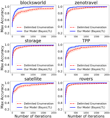
Figure 2 compares the search efficiency between our model and the delimited enumeration baseline. By employing more informed search with the MH sampler, BayesLTL discovered contrastive explanations with high accuracy with much fewer iterations and lower variance than compared to the baseline. The trend was consistent across all test domains.
Robustness to Noisy Input
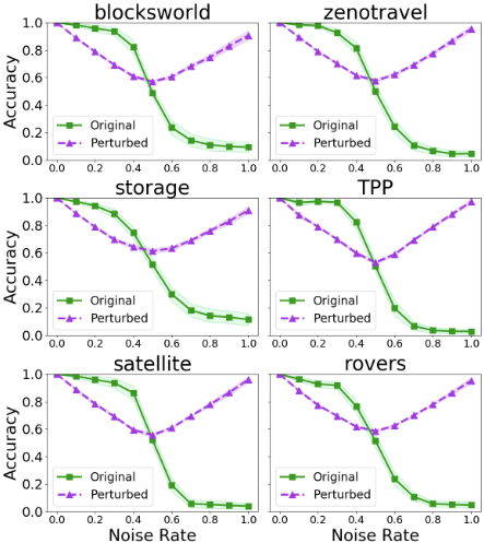
In order to test robustness, we perturbed the input X by randomly swapping traces between πA and πB. For example, a noise rate of 0.2 would swap 20% of the traces, where the accuracy of ϕground on the perturbed data, ˜X = (˜ πA, ˜ πB), would evaluate to 0.8 (note that it may be possible to discover other ϕ that achieve better accuracy on ˜X). The MAP estimates inferred from ˜X, {˜ ϕ∗ }, were evaluated on the original input X to assess any loss of ability to provide contrast.
Figure 3 shows the average accuracy of {˜ ϕ∗ }, evaluated on both ˜X and X, across varying noise rate. Even at a moderate noise rate of 0.25, the inferred ˜ ϕ∗ s were able to maintain an average accuracy greater than 0.9 on X. Such a threshold is promising for real-world applications. The robustness did start to sharply decline as noise rate increased past 0.4. For all test cases, the Neider and Gavran miner failed to generate a solution for anything with a noise rate ≥ 0.1.
Solution Space of Contrastive Explanations
Large values of M can indicate how there are often various ways to express how plan traces differ using the LTL semantics. Some LTL specifications are logically dependent. For example, the global template subsumes both the stability and the eventuality template. LTL specifications may also be related through substitutions of propositions. For example, on problems where holding a block is a prerequisite to placing it onto a table, ϕ1 = F(holding_A) ∧ F(holding_B) will be satisfied in concert with the satisfaction of ϕ2 = F(ontable_A)∧F(ontable_B). For contrastive explanation, however, one needs to be mindful of both positive and negative sides of satisfaction which affect accuracy. Relations like template subsumptions or precondition / effect pairs should not be simply favored without understanding that the converse may not hold and may result in worse accuracy.
Evaluation of LTL is trace-dependent, which depends on the domain and the problem directly. Thus, defining the metric space between two arbitrary LTL specifications is nontrivial. If such a metric space can be defined however (future work), it may integrated as part of our MH proposal function F (ϕ′ |ϕ) to sample new contrastive ϕ more efficiently.
For a contrastive ϕ, it is possible to create a new contrastive ϕ′ that includes stationary propositions or tautologies specific to the problem. For example, if ϕ1 = F(holding_A) ∧ F(holding_B) is a contrastive explanation, so is ϕ3 = F(holding_A)∧F(holding_B)∧F(earth_is_round). Our posterior distribution assigns a lower probability to ϕ3 than ϕ1 based on the decay rate on the number of conjunctions.
Also, tautologies by themselves cannot be contrastive explanations, because they can never be dissatisfied. Our model appropriately excluded such vacuous explanations.
Table 2 shows how M generally increased as |V | increased. Our premise is that multiple explanations can help in acquiring a diverse set of temporal relations, which together captures the overall behavior of a system. It permits flexibility for the human supervisor, who can flush out specifications that are deemed more or less interesting (based on personal preference or domain-specific constraints unknown apriori). However, this also opens up an interesting research direction for determining a minimal set of {ϕ} automatically. We reiterate how quantifying the distance or a notion of orthogonality between LTL formulas is an open research problem.
Evaluation on a Real-world Inspired Domain
We applied our inference model on a large force exercise (LFE) domain, which simulate air-combat games used to train pilots. Through the use of Joint Semi-Automated Forces environment [Anastasiou, 2006], realistic aircraft behavior and their state execution traces were collected for the mission objective of "gain and maintain air superiority." A total of 24 instances (i.e. traces) of LFEs were separated into positive and negative sets by a subject matter expert. The detail of the input was as follows: |πA|=16, |πB|=8, |V |=15, and the average length of traces involved 11 time steps.
Within a second (2,000 samples), our model generated ten unique contrastive explanations, all with accuracy of 0.96. ϕ∗1 = G(attrition < 0.25) ∧ G(striker not shot) represented how friendly attrition rate should be always less than 25% and that the striker aircraft should never be shot upon. ϕ∗2 = (attrition < 0.25) U (weapon release) asserted how friendly attrition rate has to be less than 25% before releasing the weapon. The model also inferred some rules of the environment, for example, asserting that propositions (attrition < 0.75) and (attrition < 0.50) precede (attrition < 0.25) (which makes sense because attrition can only increase throughout the mission). After discussion with the expert, we discovered that the model could not generate the perfect contrastive ϕground, because it required having multiple conjuncts that incorporate different LTL templates (which is not part of our defined hypothesis space). Nevertheless, the generated explanations were consistent with the expert's interpretation of achieving the mission objective of air superiority.
7 Conclusion
We have presented BayesLTL, a probabilistic Bayesian model to infer contrastive LTL specifications describing how two sets of plan traces differ. Our model generates multiple contrastive explanations more efficiently than the state-of-the-art and demonstrates robustness to noisy input. It also provides a principled approach to incorporate various forms of prior knowledge or preferences during search. It can serve as a strong foundation that can be naturally extended to multiple input sets by repeating the algorithm for all pairwise comparisons. Interesting avenues for future work include gauging the saliency of propositions, as well as deriving a minimal set of contrastive explanations.
@inproceedings{ijcai2019p776,
  title     = {Bayesian Inference of Linear Temporal Logic Specifications for Contrastive Explanations},
  author    = {Kim, Joseph and Muise, Christian and Shah, Ankit and Agarwal, Shubham and Shah, Julie},
  booktitle = {Proceedings of the Twenty-Eighth International Joint Conference on
               Artificial Intelligence, {IJCAI-19}},
  publisher = {International Joint Conferences on Artificial Intelligence Organization},
  editor    = {Sarit Kraus},
  pages     = {5591--5598},
  year      = {2019},
  month     = {8},
  note      = {Main track},
  doi       = {10.24963/ijcai.2019/776},
  url       = {https://doi.org/10.24963/ijcai.2019/776},
}
TY - CPAPER TI - Bayesian Inference of Linear Temporal Logic Specifications for Contrastive Explanations AU - Kim, Joseph AU - Muise, Christian AU - Shah, Ankit AU - Agarwal, Shubham AU - Shah, Julie T2 - Proceedings of the Twenty-Eighth International Joint Conference on Artificial Intelligence, IJCAI-19 PB - International Joint Conferences on Artificial Intelligence Organization PY - 2019 SP - 5591 EP - 5598 DO - 10.24963/ijcai.2019/776 UR - https://doi.org/10.24963/ijcai.2019/776 ER -Copied
Machine-readable versions of this paper, for tools and AI agents:





