
DDL: Deep Dictionary Learning for Predictive Phenotyping
Proceedings of the Twenty-Eighth International Joint Conference on Artificial Intelligence. AI for Improving Human Well-being. Pages 5857-5863.
https://doi.org/10.24963/ijcai.2019/812
Keywords
- Special Track on AI for Improving Human-Well Being: Health applications (Special Track on AI and Human Wellbeing)
- Special Track on AI for Improving Human-Well Being: Human wellbeing (Special Track on AI and Human Wellbeing)
- Special Track on AI for Improving Human-Well Being: AI applications for Improving Human-Well Being (Special Track on AI and Human Wellbeing)
Abstract
Predictive phenotyping is about accurately predicting what phenotypes will occur in the next clinical visit based on longitudinal Electronic Health Record (EHR) data. Several deep learning (DL) models have demonstrated great performance in predictive phenotyping. However, these DL-based phenotyping models requires access to a large amount of labeled data, which are often expensive to acquire. To address this label-insufficient challenge, we propose a deep dictionary learning framework (DDL) for phenotyping, which utilizes unlabeled data as a complementary source of information to generate a better, more succinct data representation. With extensive experiments on multiple real-world EHR datasets, we demonstrated DDL can outperform the state of the art predictive phenotyping methods on a wide variety of clinical tasks that require patient phenotyping such as heart failure classification, mortality prediction, and sequential prediction. All empirical results consistently show that unlabeled data can indeed be used to generate better data representation, which helps improve DDL's phenotyping performance over existing baseline methods that only uses labeled data.
- [Baytas et al., 2017] Inci Baytas, Cao Xiao, Xi Zhang, Fei Wang, Anil Jain, and Jiayu Zhou. Patient Subtyping via Time-Aware LSTM Networks. In Proceedings of the 23rd ACM SIGKDD International Conference on Knowledge Discovery and Data Mining, pages 65-74, Halifax, Canada, September 2017. ACM.
- [Beaulieu-Jones and Greene, 2016] Brett Beaulieu-Jones and Casey Greene. Semi-Supervised Learning of the Electronic Health Record for Phenotype Stratification. Journal of Biomedical Informatics, 64(2):168-178, October 2016.
- [Chatterji and Bartlett, 2017] Niladri Chatterji and Peter Bartlett. Alternating Minimization for Dictionary Learning with Random Initialization. In Advances in Neural Infor- mation Processing Systems, pages 1997-2006, Long Beach, USA, December 2017.
- [Choi et al., 2016a] Edward Choi, Mohammad Taha Ba- hadori, Andy Schuetz, Walter F. Stewart, and Jimeng Sun. Doctor AI: Predicting Clinical Events via Recurrent Neural Networks. In Machine Learning for Healthcare Conference, pages 301-318, Stanford, USA, May 2016. JMLR.org.
- [Choi et al., 2016b] Edward Choi, Mohammad Taha Ba- hadori, Jimeng Sun, Joshua Kulas, Andy Schuetz, and Wal- ter F. Stewart. RETAIN: An Interpretable Predictive Model for Healthcare using Reverse Time Attention Mechanism. In Advances in Neural Information Processing Systems, pages 1493-1501, Barcelona, Spain, December 2016.
- [Choi et al., 2017] Edward Choi, Mohammad Taha Bahadori, Le Song, Walter F. Stewart, and Jimeng Sun. GRAM: Graph-based Attention Model for Healthcare Representa- tion Learning. In Proceedings of the 23rd ACM SIGKDD International Conference on Knowledge Discovery and Data Mining, pages 787-795, Halifax, Canada, September 2017. ACM.
- [Choi et al., 2018] Edward Choi, Cao Xiao, Walter F. Stewart, and Jimeng Sun. MIME: Multilevel Medical Embedding of Electronic Health Records for Predictive Healthcare. In Advances in Neural Information Processing Systems, pages 4547-4557, Montreal, Canada, December 2018.
- [Dligach et al., 2015] Dmitriy Dligach, Timothy Miller, and Guergana K. Savova. Semi-Supervised Learning for Phe- notyping Tasks. In AMIA Annual Symposium Proceedings, pages 502-511, San Francisco, USA, April 2015. American Medical Informatics Association, AMIA.
- [Esteban et al., 2016] Cristóbal Esteban, Oliver Staeck, Stephan Baier, Yinchong Yang, and Volker Tresp. Pre- dicting Clinical Events by Combining Static and Dynamic Information using Recurrent Neural Networks. In IEEE In- ternational Conference on Healthcare Informatics (ICHI), pages 93--101, Xi-an, China, October 2016. IEEE Com- puter Society.
- [Hochreiter and Schmidhuber, 1997] Sepp Hochreiter and Jürgen Schmidhuber. Long Short-Term Memory. Neu- ral computation, 9(8):1735-1780, April-June 1997.
- [Ma et al., 2017] Fenglong Ma, Radha Chitta, Jing Zhou, Quanzeng You, Tong Sun, and Jing Gao. DIPOLE: Di- agnosis Prediction in Healthcare via Attention-based Bidi- rectional Recurrent Neural Networks. In Proceedings of the 23rd ACM SIGKDD International Conference on Knowl- edge Discovery and Data Mining, pages 1903-1911, Hali- fax, Canada, September 2017. ACM.
- [Ma et al., 2018] Tengfei Ma, Cao Xiao, and Fei Wang. Health-ATM: A Deep Architecture for Multifaceted Pa- tient Health Record Representation and Risk Prediction. In Proceedings of the 2018 SIAM International Conference on Data Mining, pages 261-269, San Diego, USA, May 2018. SIAM. Mairal et al., 2009]
- Julien Mairal, Francis Bach, Jean Ponce, and Guillermo Sapiro. Online Dictionary Learning for Sparse Coding. In Proceedings of the 26th Annual Interna- tional Conference on Machine Learning, pages 689-696, Montreal, Canada, June 2009. ACM.
- [Parikh and Boyd, 2014] Neal Parikh and Stephen Boyd. Proximal Algorithms. Foundations and Trends R in Opti- mization, 1(3):127-239, January 2014.
- [Tariyal et al., 2016] Snigdha Tariyal, Angshul Majumdar, Richa Singh, and Mayank Vatsa. Deep Dictionary Learning. IEEE Access, 4(1):10096-10109, April-June 2016.
References were extracted automatically from the PDF and may contain errors.
Full text extracted automatically from the PDF; figures, tables and equations may differ. The PDF is the version of record.
1 Introduction
The recent rise in popularity of deep learning (DL) and the widespread use of electronic health record (EHR) data in clinical research have sparked strong interest in using DL for electronic phenotyping, which is of paramount importance in various health analytics tasks such as chronic disease diagnosis [Ma et al., 2017], patient sub-typing [Baytas et al., 2017] and disease prediction [Esteban et al., 2016]. The key advantage of DL models are their abilities to construct deep features that capture complex and long-range data dependencies efficiently, both of which are particular traits of biomedical data. This helps DL models achieve better performance and require less effort in feature engineering than classical machine learning (ML) models.
Despite these successes, the training of DL-based phenotyping models often relies on direct supervision via labeled data, which in turn requires access to a large volume of EHR data annotated with relevant medical labels. This highlights a key weakness of existing DL-based phenotyping models in terms of practical efficiency and data utilization. First, acquiring labeled data is often prohibitively expensive due to the incurred labor-intensive data annotation, which makes the training practically inefficient. Second, most DL models are trained using supervised learning methods, which do not make use of unlabeled EHR data [Choi et al., 2016b; Ma et al., 2017; Ma et al., 2018]. Ignoring unlabeled data, however, leads to a severe under-utilization of available information since such data can still be exploited to learn a better representation of labeled data (hence, better prediction performance) even though they do not contain predictive information. To mitigate the above weaknesses, this paper aims to develop a deep dictionary learning (DDL) framework that utilizes and combines both labeled and unlabeled data to learn a better data representation for predictive phenotyping.
∗Tianfan Fu and Trong Nghia Hoang contribute equally.
To elaborate, DDL implements a hybrid learning architecture that combines ideas from both dictionary learning and recurrent neural network (RNN) for temporal prediction. This is achieved by first embedding raw, unlabeled EHR data into a latent feature space using DDL's RNN component. Then, dictionary learning is applied on the resulting set of embedded representations to search for a smaller set of patterns that occur frequently across different patients' representations. This in turn allows DDL to characterize each patient's embedded representation as a linear combination of those frequent patterns, which constitutes their deep dictionary representations (Section 2.2).
Furthermore, to optimize the above deep dictionary representation, DDL develops a deep dictionary decoder that reconstructs a patient's unlabeled EHR data from its deep dictionary representation. This is achieved by minimizing the decoder's reconstruction loss, which helps establish a parsimonious set of hidden-layer patient prototypes (Section 2.3). Different patients can then be viewed as different combinations of these prototypes where the combination coefficients represent its high-level feature description. These coefficients are then coupled with the patients' labeled data to learn a mapping from each patient's high-level description to his/her target outcomes (Section 2.4). This is also demonstrated in our experiments (Section 3) that such representation indeed induces better performance than those of the existing baselines for predictive phenotyping.
Last but not least, DDL also develops an end-to-end training
mechanism that optimizes the above data embedding (Section 2.2), reconstruction (Section 2.3) and prediction (Section 2.4) components simultaneously. This intuitively allows DDL's representation components (built with unlabeled data) to coordinate with its prediction component (built with labeled data) to avoid generating representations which are biased towards artifacts in unlabeled data. As a result, DDL generates a less biased representation that is beneficial for both reconstruction and prediction loss minimization, thus leading to better predictive phenotyping performance. This is in contrast to existing semi-supervised ML methods [Mairal et al., 2009; Tariyal et al., 2016; Dligach et al., 2015], which perform training with separate supervised and unsupervised steps, and are therefore vulnerable to biased representations caused by artifacts in unlabeled data.
To demonstrate the aforementioned advantages of DDL, we evaluated its performance and compared it against those of a set of selected state-of-the-art predictive phenotyping baselines on an extensive benchmark (Section 3) comprising multiple real-world EHR datasets and a wide variety of predictive phenotyping tasks (e.g., heart failure classification, mortality and sequential prediction). The reported results demonstrate improved prediction performance of DDL consistently over all baselines, which provides strong empirical evidence to support our key contribution statement that unlabeled data can be coupled with labeled data via semi-supervised learning to boost the performance of predictive phenotyping.
2 Method
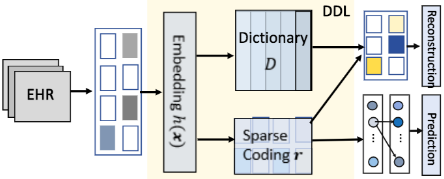
This section presents the technical details of our developed DDL framework. In particular, our notations are first introduced in Section 2.1. Section 2.2 presents our developed deep dictionary encoder that generates deep dictionary representations for EHR data. Section 2.3 then presents a deep dictionary decoder that maps the generated deep dictionary representations back to EHR data, and optimizes it via minimizing the reconstruction loss. Section 2.4 develops a deep dictionary predictor that maps each patient's deep dictionary representation to relevant target outcomes. Finally, Section 2.5 presents a collaborative training architecture (see Fig. 1) that jointly trains all the aforementioned components, thus allowing them to converge on the best deep dictionary representation that minimizes both reconstruction and prediction losses.
2.1 Notations and Definitions
Our EHR data comprises medical records of N different patients. The medical record of each patient n = 1 . . .N is represented as: the input Xn ≜ [x(1) n ; x(2) n ; · · · ; x(kn) n ] denotes a collection of patient's records for his/her past visits to the clinic, and kn is the number of the n-th patient's visits. Each visit record x(i) n ∈ {0, 1}p can be represented as a multihot vector that indicates whether the patient was associated with a particular medical code during his/her i-th visit to the clinic. There are p unique medical codes. The corresponding output/label yn ∈ {0, 1}c of a patient's EHR data Xn is also a multi-hot vector that indicates whether the patient was diagnosed with a certain target disease or condition. There are c unique target diseases or conditions. In our setting, the label yn is only available for a small subset of M < N patients with n = 1, . . . ,M, which is designated as our labeled training dataset D ≜ (Xn, yn)Mn=1 . Given the labeled and unlabeled EHR datasets of previous patients, i.e. D ≜ (Xn, yn)Mn=1 and U ≜ (Xn, )Nn=1 , respectively, the aim of the predictive phenotyping task is to learn a latent function that maps from a patient's EHR data X to an output vector y ∈ {0, 1}c that characterizes his/her phenotype accurately.
2.2 Deep Dictionary Encoder
This section develops a deep dictionary encoder that can succinctly captures embedded representations from the patient's unlabeled EHR data U = (Xn)Nn=1 coherently and in accordance with each other. This will help establish a parsimonious set of hidden-layer patient prototypes, which constitutes our deep dictionary representation. This can be achieved by combining ideas from both deep and dictionary learning, which is an emerging paradigm of predictive deep models in computer vision.
Intuitively, the key idea is to first exploit the capability of DL model to embed complex data (e.g., EHR data with varying length due to different numbers of clinical visits among different patients) into fixed-size, low-level embeddings. To incorporate high-level representations for better predictive performance, we use dictionary learning to further decompose these embeddings into fundamental patterns that succinctly characterize a space of high-level features. The patient embeddings can then be projected onto this space and the projection coefficients can be leveraged as high-level features to improve the cognitive capability of the predictive model.
To represent each patient, we employ an RNN with Long Short Term Memory (LSTM) architecture [Hochreiter and Schmidhuber, 1997], which is well-known for its ability to capture long-range dependencies within longitudinal data such as patient's EHR. In particular, the LSTMmodule generates a latent embedding gn from the multi-hot encoded patient record Xn,
where gn ∈ Rd is the output of the LSTM, which is used as the embedded, fixed-length patient representation. In the above equation, we concatenate the multi-hot vectors (corresponding to the patient's different clinical visits) into an extended input vector for the LSTM. Based on the above embedded representation, we further adopt dictionary learning to extract both a dictionary of hidden-layer prototypes (which is patient-independent) and a collection of weight vectors (one per patient), which specifies how these prototypes can be combined to characterize a particular patient accurately. This is achieved via minimizing the following regularized projection loss,
with respect to {rn}Nn=1 (rn ∈ Rk ) and D ∈ Rd×k , which denote the weight vectors (or sparse codes) that characterize each patient and the dictionary of patient prototype represented in the embedded space, respectively. To avoid generating trivial solutions, the above loss is also regularized by penalizing the complexities λ1‖rn‖1 and λ2‖D‖2F of the sparse codes and dictionary with λ1 and λ2 being the regularization parameters. The embedded patient prototype can then be mapped back to the patient space via a deep dictionary decoder (see Section 2.3). Note that the above loss in Eq. 2 is convex in D given {rn}Nn=1 and vice versa. Thus, Eq. 2 can be optimized (with local convergence guarantee) via alternating minimization [Chatterji and Bartlett, 2017].
2.3 Deep Dictionary Decoder
To map the patient deep dictionary representation (D, rn) back to the original patient space, we develop a deep dictionary decoder module which specifically maps (D, rn) to a vector qn ≜ [q(1) n . . . q(p) n ] ∈ [0, 1]p of probability scores such that q(i) n ∈ [0, 1] denotes the probability that medical code i contributes actively to the patient's predicted outcome yn. We parameterize the decoder D(D, rn) as a neural network with a fully-connected layer followed by a sigmoid activation,
where the sigmoid operator σ(x) ≜ 1/(1 + exp(-x)) is applied point-wise to each element of the logit vector WDrn. The above neural network is parameterized by the weight W of the dense, fully-connected layer. To optimizeW, we generate the augmented dataset {(D, rn), Xn}Nn=1 , which can be generated via the deep dictionary embedding technique presented in Section 2.2. The augmented dataset can then be used to train the above neural network via back-propagation with the following cross-entropy reconstruction loss,
where X(i) n ∈ [0, 1] is the average occurrence of medical code i over all clinical visits of patient n. Optimizing Eq. 4 thus yields the deep dictionary decoder. To use this deep dictionary decoder on an unseen patient, we project the patient embedded representation g on D via minimizing ‖g-Dr‖22 with respect to r, which can be solved analytically.
2.4 Deep Dictionary Predictor for Labeled Data
Given the deep dictionary representation (D, rn) of labeled training data D = (Xn, yn)Mn=1 , we can further build a deep dictionary predictor that maps from a patient's sparse code rn to a vector on of predicted probabilities that the patient will be associated with each target outcomes (e.g., disease or mortality). This is achieved by parameterizing the predictor with a fully-connected layer followed by a soft-max activation,
where V ∈ Rc×k and b ∈ Rc are the weight matrix and bias vector, respectively. These parameters can then be learned via minimizing the cross-entropy between the predicted probabilities on and the ground-truth label yn,
with respect to V and b. c is number of prediction targets, and n = 1 . . .M is the patient index in the labeled training data D with yn ∈ {0, 1}c denote the corresponding patient label characterizing his/her phenotype. y(i) n and o(i) n are the i-th entries of yn and on, respectively.
2.5 Collaborative Prediction and Reconstruction
This section develops an collaborative architecture that connects the previously developed deep dictionary decoder and deep dictionary predictor using a common layer of deep dictionary encoder (see Fig. 1).
This allows us to optimize the above components simultaneously so that the deep dictionary encoder could interact with both the decoder and predictor modules to figure out a viable communication medium (i.e., the dictionary) that allows them to reach a consensus. Intuitively, the encoder plays the role of a mediator that suggests communication options for the decoder and predictor, and depending on the resulting quality of communication between them (i.e., the incurred prediction and reconstruction losses), the encoder will revise the communication medium until it facilitates an acceptable consensus between the decoder and predictor. This is in contrast to a naive solution that trains these components separately, which does not allow communication/coordination between the encoder, decoder and predictor; and therefore, cannot guarantee that the learned results would be optimized for both reconstruction and prediction.
To facilitate the aforementioned coordination, we aggregate the loss functions of these components (i.e., encoder, decoder and predictor) to generate a combined performance feedback, which can be exploited to update them jointly via stochastic gradient back-propagation,
Algorithm 1 DDL (Tmax - max no. of optimizing iterations)
- 1: Input: randomized LSTM,W, D, V and b. 2: for t = 1 . . . Tmax do 3: sample mini-batchM⊆ {X1, . . . ,XN}. 4: for Xn ∈ M do 5: Encoder: Estimate Embedded Representation 6: gn←LSTM(Xn) = LSTM (x(1) n , x(2) n , . . . , x(kn) n ) 7: Encoder: Estimate Sparse Code Representation 8: rn ← arg min r∈Rk ‖gn - Dr‖22 + λ1‖r‖1 using Alg. 2. 9: Decoder: Reconstruction Data 10: qn ← D(D, rn;W) via Eq. 3 11: Predictor: Estimate Prediction Probabilities 12: if Xn ∈ D (i.e., Xn is labeled) then 13: on ← softmax (Vrn + b) via Eq. 5 14: end if 15: end for 16: Compute L's stochastic gradient using the above 17: Update all parameters via stochastic gradient descent. 18: end for 19: Output: optimized LSTM,W, D, V and b.
where Lℓ is parameterized byW,D,V, b and {rn}Nn=1 for which the projection loss Ld only depends on (D, {rn}Nn=1 ), the reconstruction loss Lc depends on (W,D, {rn}Nn=1 ), and the prediction loss Lc depends on (V, b, {rn}Mn=1 ). The extra hyper-parameters ηd, ηr and ηc are manually tuned to trade-off between individual losses.
In addition, note that the projection and reconstruction losses do not depend on the training output and can therefore be pre-trained in advance using only unlabeled data U. In this case, the loss function reduces to
which is first minimized (using unlabeled data) with respect to D,W and {rn}Nn=1 to generate a good starting point for these parameters before further optimizing them via Eq. 7, and in accordance with the predictor's parameters (V, b) using labeled data, thus still allowing end-to-end training that simultaneously optimizes both the supervised and unsupervised components of DDL (albeit with a starting point generated from pre-training its unsupervised component). The above process is, however, not computationally efficient due to the large number of optimizing parameters, which consequently results in a very slow convergence rate if we train all these parameters from scratch. To address this issue, we instead adopt a different approach which first computes a warm-start for the sparse codes {rn}Nn=1 (as detailed below) as a good starting point to initiate gradient back-propagation on the entire network. The main algorithm is shown in Algorithm 1.
To initialize the sparse code rn for each patient, we fix the dictionary D and the data embedding layer of the network (hence, the patient's embedding representation gn). Thus, given (D, gn), the objective in Eq. 7 is convex with respect to rn and reduces the following form,
which can be solved efficiently using proximal gradient method [Parikh and Boyd, 2014], as detailed in Algorithm 2 below. The use of proximal gradient descent is a technical necessity in this context since (9) is not differentiable everywhere due to the L1 regularization λ1‖r‖1. Proximal gradient descent sidesteps this issue by decomposing (9) into two parts: (a)differentiable f(r) ≜ 1/2‖gn -Dr‖22 , and (b)nondifferentiable h(r) ≜ λ1‖r‖1. Thus, starting from a random initialization of r, we can use gradient descent on the first part to update r with respect to the differentiable part f(r) and then update it with respect to the non-differentiable part λ1‖r‖1 via the following proximal operator,
which can be solved analytically. Interested readers are referred to [Parikh and Boyd, 2014] for further details.
3 Experiment
In this section, we empirically evaluate the performance of DDL against several state-of-the-art baseline methods on 3 healthcare datasets, Heart Failure (HF) [Ma et al., 2018], MIMIC-III and a subset of Truven MarketScan Data 1 , which contain 16794, 58000 and 72179 EHR samples, respectively. The numbers of clinical variables (p) in HF, MIMIC-III and TRUVEN are 1865, 283 and 283, respectively. In HF and MIMIC-III, the task is to predict the HF and mortality binary outcomes. For TRUVEN data, the prediction task is to predict which clinical variables are positive in the patient's latest visit given data of his/her past visits.
3.1 Experiment Settings
For each experiment, we randomly generate 5 different partitions of the entire dataset into training, validation and testing sets with a 7 : 1 : 2 ratio. The reported result of each tested method is its averaged result over 5 independent runs corresponding to the 5 different data partitions. Our method is implemented by Tensorflow 1.9.0 and Python 3.5 2 ; and tested on an Intel Xeon E5-2690 machine with 256G RAM and 8 NVIDIA Pascal Titan X GPUs. We evaluate each method
1 https://marketscan.truvenhealth.com/
2 Code is available at https://github.com/futianfan/dictionary.
Algorithm 2 Proximal Optimization (r, Tmax)
- 1: Initialize learning rates ξ 1 , . . . , ξ Tmax
- 2: for k = 1 . . . Tmax do
- 3: r = r - ξ k∇rf(r) = r - ξ kD⊤(g -Dr)
- 4: r = proxξk λ1h (r)
- 5: if converge then
- 6: break
- 7: end if
- 8: end for
(b)
(c)
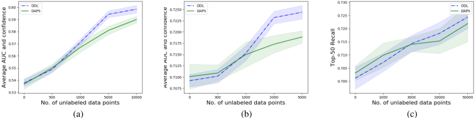
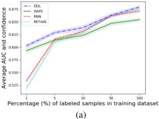
Figure 3: Graphs of average accuracy (with 95% confidence interval) of DDL and baseline methods on (a) HF, (b) MIMIC-III, and (c) TRUVEN datasets. In all experiments, the size of training dataset is fixed while the fraction of labeled data is being varied.
using its best fine-tuned hyper-parameter configurations. The best configurations of DDL are described below.
For HF dataset, the no. of hidden units of DDL's RNN component is set to 100. Its dictionary size is set to 10. Its learning rate for gradient back-propagation on the aggregate loss (Eq. 7) is set to be 1e-2. To trade-off between projection, reconstruction and prediction losses, we set ηd = 1e - 1, ηc = 1 and ηr = 1e - 3 in Eq. 7. For the projection loss Ld in Eq. 2, the regularization hyper-parameters are set as λ1 = 5e-2 and λ2 = 1e-3. For MIMIC-III dataset, we use the same configuration but with the following minor changes on learning rate (5e - 2) and trade-off coefficients (ηd = ηc = 1 and ηr = 2e - 3) between individual losses of DDL. For TRUVEN dataset, we also use the similar configuration but with the dictionary and RNN component's hidden sizes set to be 15 and 200, respectively. In addition, the trade-off coefficients in Eq. 7 are also adjusted to ηd = 1e - 1 and ηc = ηr = 1. The batch sizes of DDL's stochastic gradient descent on HF and MIMIC-III are both set to be 32, while on TRUVEN, it is set to be 64 (since TRUVEN dataset is larger than the others).
3.2 Baseline Methods
To demonstrate the advantage of DDL, we evaluate and compare its performance with those of the baseline methods, which includes (a) state-of-the-art deep phenotyping methods such as Doctor-AI (RNN) [Choi et al., 2016a], Reverse Time Attention RNN (RETAIN) [Choi et al., 2016b], Denoising Autoencoders for Phenotype Stratification (DAPS) [BeaulieuJones and Greene, 2016], and (b) two traditional ML methods featuring Logistic Regression (LR) with L2 regularizer and Dictionary Learning (DictLearn) [Mairal et al., 2009]. The LR, DictLearn and DAPS baselines were trained using the aggregated feature vector ˜Xn ∈ {0, 1}p (instead of using the original input Xn), which was derived from the original EHR data Xn such that ˜X(i) n = 1 if the i-th clinical variable occurred at least once in Xn's multiple clinical visit. Otherwise, ˜X(i) n = 0. Furthermore, we also include a simplified version of DDL that excludes the decoder module.
| Model | HF | MIMIC-III |
|---|---|---|
| LR DictLearn DAPS RNN RETAIN | 0.636 ± 0.003 | 0.763 ± 0.004 |
| 0.634 ± 0.004 | 0.771 ± 0.006 | |
| 0.651 ± 0.002 | 0.794 ± 0.004 | |
| 0.668 ± 0.004 | 0.807 ± 0.004 | |
| 0.675 ± 0.003 | 0.817 ± 0.004 | |
| DDL | 0.682±0.004 | 0.819±0.004 |
| DDL w.o. decoder | 0.669 ± 0.006 | 0.813 ± 0.004 |
| Model | HF | MIMIC-III |
|---|---|---|
| LR | 34.3 ± 2.1 | 21.2 ± 1.9 |
| DictLearn | 49.3 ± 2.9 | 31.2 ± 3.0 |
| DAPS | 125.0 ± 5.6 | 86.4 ± 2.3 |
| RNN | 64.6 ± 8.4 | 25.6 ± 3.2 |
| RETAIN | 100.7 ± 10.1 | 79.4 ± 14.3 |
| DDL | 234.4 ± 21.3 | 178.3 ± 11.0 |
| DDL w.o. decoder | 183 ± 14.1 | 128.3 ± 6.0 |
| Model | Top-50 recall | Top-30 recall | Time |
|---|---|---|---|
| LR | 0.753 ± 0.002 | 0.605 ± 0.002 | 43.0 ± 1.2 |
| DictLearn | 0.752 ± 0.002 | 0.610 ± 0.002 | 84.2 ± 2.0 |
| DAPS | 0.773 ± 0.003 | 0.621 ± 0.002 | 232 ± 34 |
| RNN | 0.783 ± 0.003 | 0.630 ± 0.002 | 113.0 ± 8.2 |
| RETAIN | 0.786 ± 0.007 | 0.632 ± 0.005 | 134.4 ± 12.0 |
| DDL | 0.791 ± 0.004 | 0.634 ± 0.003 | 624 ± 34 |
| DDL w.o. decoder | 0.780 ± 0.05 | 0.627 ± 0.005 | 427 ± 31 |
3.3 Comparison in Supervised Setting
This section evaluates and reports the performance of DDL and baseline methods in supervised setting. That is, the training only uses EHR data with label. For experiments on HF and MIMIC-III datasets, the performance of each method is measured by the standard ROC-AUC (Area Under the Receiver Operating Characteristic Curve) score for binary classification where higher score implies better performance. For TRUVEN datasets, the final prediction is generated by combining the results of individual binary classification tasks (one for each variable in the patient's last clinical visit). In particular, the top k variables with largest predicted probabilities to be positive are treated as positive labels while the others are associated with negative labels in our multi-label prediction. Thus, the performance of each method on TRUVEN dataset is measured using the following top-k recall metric:
The averaged performance (with standard deviation) over 5 different runs of all tested methods are reported in Table 1 for HF and MIMIC-III datasets, and in Table 3 for TRUVEN dataset. The incurred training time for all methods are reported in Table 2. The reported results shown that: (1) DDL consistently outperforms all baseline methods in terms of prediction accuracy (ROC-AUC) on all datasets, which demonstrates the advantage of using a hybrid deep dictionary learning in predictive phenotyping; (2) among the baselines, DL-based methods perform significantly better than traditional ML baselines such as LR and DictLearn, which justifies the choice of using DL as the base model (in our framework) to be combined with dictionary learning; and (3) DDL with decoder achieved better results than DDL without decoder, thus supporting our statement earlier that jointly training both supervised and unsupervised components (instead of training them separately) allow them to coordinate on a better data representation.
3.4 Comparison in Semi-Supervised Setting
To showcase the advantage of leveraging unlabeled data, we design two scenarios to demonstrate it empirically. In the first scenario, we fix the number of labeled data samples and observe the changes in DDL's and baseline methods' performance when the number of unlabeled data samples varies. The results are plotted in Figure 2, which show the tested methods' average prediction accuracies of 3 independent runs and their confidence intervals. It can be observed that across all datasets, the prediction performance increases as more unlabeled data is used for training, thus supporting our claim earlier that unlabeled data can be exploited as an extra source of information to improve performance of predictive phenotyping models.
In the second scenario, we fix the total number of training data samples while varying the percentage of labeled samples within the training set, and observe how the tested methods' performance changes accordingly. From the results in Figure 3 above, it shows that DDL outperforms other methods most significantly when the amount of labeled data is limited: when this happens, the performance of RNN and RETAIN degrade the most since they cannot make use of unlabeled data. DAPS on the other hand can leverage unlabeled data and performs better than RNN and RETAIN but still worse than DDL since it does not train both supervised and unsupervised components, thus being vulnerable to artifacts in unlabeled data.
4 RelatedWorks
In this section, we briefly discuss the success use of deep learning in predictive phenotyping. [Choi et al., 2016a] used Recurrent Neural Network (RNN) to modelling temporal data in Electronic Health Record (EHR). [Choi et al., 2016b; Ma et al., 2017; Choi et al., 2017] uses attention mechanisms to detect important visits and clinical variables. [Choi et al., 2018] utilized multilevel structures to modelling EHR data in a finer-grained manner. [Ma et al., 2018] extracts comprehensive patient pattern via using time-aware neural architectures.
5 Conclusion
This paper addressed the label-insufficiency issue in predictive healthcare where unlabeled data are abundant but labeled data is limited. To combine both labeled and unlabeled data for better predictive performance, we propose a deep dictionary learning (DDL) framework that utilizes unlabeled data to learn more generalizable representation of data for the predictive model. For example DDL was evaluated on real-world healthcare datasets (MIMIC-III, Heart Failure and Truven) for disease prediction. The results consistently show that the representations learned from unlabeled data generalize better and improve the predictive accuracy.
Acknowledgements
This work was supported by the National Science Foundation award IIS-1418511, CCF-1533768 and IIS-1838042, the National Institute of Health award 1R01MD011682-01 and R56HL138415.
@inproceedings{ijcai2019p812,
  title     = {DDL: Deep Dictionary Learning for Predictive Phenotyping},
  author    = {Fu, Tianfan and Hoang, Trong Nghia and Xiao, Cao and Sun, Jimeng},
  booktitle = {Proceedings of the Twenty-Eighth International Joint Conference on
               Artificial Intelligence, {IJCAI-19}},
  publisher = {International Joint Conferences on Artificial Intelligence Organization},
  editor    = {Sarit Kraus},
  pages     = {5857--5863},
  year      = {2019},
  month     = {8},
  note      = {AI for Improving Human Well-being},
  doi       = {10.24963/ijcai.2019/812},
  url       = {https://doi.org/10.24963/ijcai.2019/812},
}
TY - CPAPER TI - DDL: Deep Dictionary Learning for Predictive Phenotyping AU - Fu, Tianfan AU - Hoang, Trong Nghia AU - Xiao, Cao AU - Sun, Jimeng T2 - Proceedings of the Twenty-Eighth International Joint Conference on Artificial Intelligence, IJCAI-19 PB - International Joint Conferences on Artificial Intelligence Organization PY - 2019 SP - 5857 EP - 5863 DO - 10.24963/ijcai.2019/812 UR - https://doi.org/10.24963/ijcai.2019/812 ER -Copied
Machine-readable versions of this paper, for tools and AI agents:





