On Causal Identification under Markov Equivalence

1 Introduction

A prominent approach to infer causal effects leverages a combination of substantive knowledge about the domain under investigation, usually encoded in the form of a causal diagram, with observational data [Pearl, 2000; Bareinboim and Pearl, 2016]. A sample diagram is shown in Fig. 1a, where the nodes represent variables, directed edges represent direct causal relations from tails to heads, and bi-directed arcs represent the presence of unobserved (latent) variables that generate spurious association between the variables. The decision problem of whether an interventional distribution can be computed from a combination of observational and experimental data together with the causal diagram is known as the problem of identification of causal effects (identification, for short). For instance, a possible task is to identify the effect of do(X=x) on V4=v4, i.e. Px(v4), given the diagram in Fig. 1a and data from the distribution P (X, V1, ..., V4).

This problem has been extensively studied in the literature with a number of criteria established [Pearl, 1993; Galles and Pearl, 1995; Kuroki and Miyakawa, 1999; Tian and Pearl, 2002; Huang and Valtorta, 2006; Shpitser and Pearl, 2006; Bareinboim and Pearl, 2012], which include the back-door criterion and the do-calculus [Pearl, 1995]. Despite their power, these techniques require a fully specified causal diagram, which is not always available in practical settings.

∗This is an abridged version of [Jaber et al., 2018a] which won the best student paper award at UAI-18 and [Jaber et al., 2019].

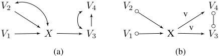
One may try to learn the causal diagram from data. However, it is common that only an equivalence class of causal diagrams can be consistently inferred from observational data [Verma, 1993; Spirtes et al., 2001]. A useful representation of such an equivalence class is a partial ancestral graph (PAG) [Zhang, 2008b]. Fig. 1b shows the PAG that can be inferred from observational data generated by Fig. 1a. In PAGs, directed edges signify (possibly indirect) causal relations and circle marks indicate structural uncertainty.

In this work, we analyze the marriage of these two lines of investigation. Identification from an equivalence class is considerably more challenging than from a single diagram due to the structural uncertainty regarding both the causal relations among the variables and the presence of hidden variables. Zhang [2007] extended the do-calculus to PAGs. In practice, however, it is computationally hard to decide whether there exists a sequence of applications of the rules of the generalized calculus to identify an effect. Perkovi´c et al. [2015] generalized the back-door criterion to PAGs, and provided a complete algorithm to find a back-door admissible set, should such a set exist. However, in practice, no adjustment set exists for many identifiable effects. In this extended abstract, we summarize the approach taken in [Jaber et al., 2018b; Jaber et al., 2018b; Jaber et al., 2019] that culminated in a complete algorithm to identify causal effects given PAGs. Specifically, our contributions are as follows:

1. We revisit the original identification algorithm given causal diagrams and introduce a new formulation which is more amenable under structural uncertainties.
2. We derive crucial PAG properties including a novel graph-decomposition strategy that breaks a target causal distribution into an equal product of more tractable ones.
3. We develop a complete algorithm to compute the effect of an arbitrary set of intervention variables on an arbitrary outcome set from a PAG and observational data.

2 Preliminaries

In this section, we introduce the basic notation and machinery used throughout the paper. Bold capital letters denote sets of variables, while bold lowercase letters stand for particular value assignments to those variables.

2.1 Structural Causal Models

We use the language of Structural Causal Models (SCM) [Pearl, 2000, pp. 204-207] as our basic semantic framework. Formally, an SCM M is a 4-tuple 〈U,V,F, P(U)〉, where U is a set of exogenous (latent) variables and V is a set of endogenous (measured) variables. F represents a collection of functions {fi} such that each endogenous variable Vi ∈ V is determined by a function fi ∈ F, where fi is a mapping from the respective domain of Ui ∪ Pai to Vi, Ui ⊆ U, Pai ⊆ V \ {Vi}. The uncertainty is encoded through a probability distribution over the exogenous variables, P(U), and the marginal distribution induced over the endogenous variables P(V) is called observational. Every SCM is associated with one causal diagram where every variable Vi ∈ V is a node, and there exists a directed edge from every node in Pai to Vi. Also, for every pair Vi, Vj ∈ V such that Ui ∩ Uj ̸= ∅, there exists a bi-directed edge between Vi and Vj . We restrict our study to recursive systems, which means that the corresponding diagram will be acyclic.

Within the structural semantics, performing an action X= x is represented through the do-operator, do(X =x), which encodes the operation of replacing the original equation for X by the constant x and induces a submodel Mx. The resulting distribution is denoted by Px, which is the main target for identification in this paper. For further details on structural models, we refer readers to [Pearl, 2000].

2.2 Ancestral Graphs

We now introduce a graphical representation of equivalence classes of causal diagrams. A mixed graph can contain directed and bi-directed edges. A is an ancestor of B if they share a directed path out of A. A is a spouse of B if A ↔ B is present. An almost directed cycle happens when A is both a spouse and an ancestor of B. An inducing path is a path on which every node (except for the endpoints) is a collider on the path (i.e., both edges incident to X are into X) and every collider is an ancestor of an endpoint of the path. A mixed graph is ancestral if it doesn't contain a directed or almost directed cycle. It is maximal if there is no inducing path between any two non-adjacent nodes. A Maximal Ancestral Graph (MAG) is a graph that is both ancestral and maximal [Richardson and Spirtes, 2002].

In short, a MAG represents a set of causal diagrams that entail the same independence and ancestral relations among the observed variables. Different MAGs may be Markov equivalent in that they entail the exact same independence model. A partial ancestral graph (PAG) represents an equivalence class of MAGs [M], which shares the same adjacencies as every MAG in [M] and displays all and only the invariant edge marks. A circle indicates an uncommon edge mark. A PAG is learnable from the conditional independence relations among the observed variables and the FCI algorithm is a standard method to learn such an object [Zhang, 2008b].

2.3 Graphical Notions

Given a causal diagram, a MAG, or a PAG, a path between X and Y is potentially directed (causal) fromX to Y if there is no arrowhead on the path pointing towards X. X is a possible ancestor of Y , i.e., X ∈ An(Y ), if there is a potentially directed path from X to Y . By stipulation, X ∈ An(X). Y is called a possible child of X, i.e. Y ∈ Ch(X), if they are adjacent and the edge is not into X. For a set of nodes X, we have Ch(X) = ∪X∈XCh(X). If the edge marks on a path between X and Y are all circles, we call the path a circle path. We refer to the closure of nodes connected with circle paths as a bucket. Obviously, given a PAG, nodes are partitioned into a unique set of buckets.

A directed edge X → Y in a MAG or PAG is visible if there exists no causal diagram in the corresponding equivalence class where there is an inducing path between X and Y that is into X. This implies that a visible edge is not confounded (X ←-→ Y doesn't exist). Which directed edges are visible is easily decidable by a graphical condition [Zhang, 2008a, Def. 8], so we simply mark visible edges by v. For brevity, we refer to any edge that is not a visible directed edge as invisible.

3 Revisit Identification in Causal Diagrams

Tian and Pearl [2002] presented an identification algorithm based on a decomposition strategy of the causal diagram into a set of so-called c-components (confounded components).

Definition 1 (C-Component). In a causal diagram, two nodes are said to be in the same c-component if and only if they are connected by a bi-directed path, i.e., a path composed solely of bi-directed edges.

For any set C ⊆ V, the quantity Q[C] is defined to denote the post-intervention distribution of C under an intervention on V \ C, i.e. Pv\c(c). Given a diagram D, Q[C] decomposes into a product of sub-queries over the c-components in DC, where DC denotes the (induced) subgraph of D over C. Hence, we get the following decomposition, where Ci is a c-component in DC:

The significance of c-components and their decomposition is evident from [Tian, 2002, Lemmas 10, 11], which are the basis of Tian's identification algorithm. Our goal is to reformulate the procedure with a more local, atomic criterion shown in Lem. 1. The step-wise algorithm is shown in Alg. 1.

Lemma 1. Given a causal diagram D over V, X ∈ T ⊆ V, and Pv\t, i.e., an expression for Q[T]. If X is not in the same c-component with a child in DT, then Q[T \ {X}] is identifiable and given by

where SX is the c-component of X in DT and Q[SX ] is computable from Pv\t by [Tian, 2002, Lemma 11].

Algorithm 1 ID(x, y) given Causal Diagram G

• Input: two disjoint sets X,Y ⊂V Output: Expression for Px(y) or FAIL 1: Let D= An(Y)GV\X 2: Let the c-components of GD be Di, i = 1, . . . , k 3: Px(y) = ∑d\y ∏i IDENTIFY(Di,V, P) 4: function IDENTIFY(C, T, Q = Q[T]) 5: if C = T then return Q[T] /* Let SB denote the c-component of {B} in GT */ 6: if ∃B ∈ T \ C such that SB ∩ Ch(B) = ∅ then 7: Compute Q[T \ {B}] from Q; ▷ Lemma 1 8: return IDENTIFY(C, T \ {B}, Q[T \ {B}]) 9: else 10: throw FAIL

The revised algorithm requires checking an atomic criterion at every instance of the recursive routine IDENTIFY. This might not be crucial when the precise causal diagram is known and the induced subgraphs preserve complete information about the c-components and the ancestral relations between the nodes. However, it becomes significant when the domain description is an equivalence class represented by a PAG, in which structural information is partial.

4 PAG Properties and Q-Decomposition

Evidently, induced subgraphs of the original causal diagram play a critical role in identification (cf Alg. 1). It is natural to expect that in the generalized setting we study here, induced subgraphs of the given PAG will also play an important role. An immediate challenge, however, is that a subgraph of a PAG P over V induced by A ⊆ V is, in general, not a PAG that represents a full Markov equivalence class. In particular, if D is a diagram in the equivalence class represented by P, PA is in general not the PAG that represents the equivalence class of DA. For example, let D and P denote the diagram and the corresponding PAG in Figure 1, respectively, and let A = {V1, V2, X, V4}. Then, V4 is disconnected in DA while it is a child of X in PA. Despite this subtlety, we establish a few facts showing that for any A ⊆ V and any diagram D in the equivalence class represented by P, some information about DA, which is particularly relevant to identification, can still be read off from PA. In [Jaber et al., 2018a], we discuss a key property related to c-components.

Definition 2 (PC-Component). In a MAG, a PAG, or any induced subgraph thereof, two nodes are in the same possible c-component (pc-component) if there is a path between them such that (1) all non-endpoint nodes along the path are colliders, and (2) none of the edges is visible.

As mentioned earlier, a c-component in a causal diagram plays a central role in identification. The following proposition establishes a graphical condition in an induced subgraph PA that is necessary for two nodes being in the same c-component in DA for some diagram D represented by P.

Proposition 1. Let P be a PAG over V, and D be any causal diagram in the equivalence class represented by P. For any X, Y ∈ A ⊆ V, if X and Y are in the same c-component in DA, then X and Y are in the same pc-component in PA.

This result provides a sufficient condition for not belonging to the same c-component in any of the induced causal diagrams. In the aforementioned PA of Fig. 1b, for example, V1 and V4 or X and V4 are not in the same pc-component, which implies by Prop. 1 that they are not in the same c-component in DA for any D in the equivalence class represented by the PAG in Fig. 1b. As a special case of Def. 2, we define the following notion, which will prove useful later on.

Definition 3 (DC-Component). In a MAG, a PAG, or any induced subgraph thereof, two nodes are in the same definite c-component (dc-component) if they are connected with a bidirected path, i.e. a path composed of bi-directed edges.

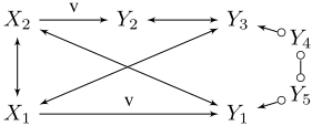
Next, we use the pc-component property to devise a decomposition for Q[C] in PAGs akin to that for causal diagrams presented in Eq. 1. However, the decomposition in PAGs is challenging due to the structural uncertainties; most relevant the presence of latent confounders. For instance, given the query Q[Y] over the PAG in Fig. 2, the sequence of nodes 〈Y2, Y3, Y4, Y5, Y1〉 is connected with invisible edges, which are possibly confounded. Hence, any naive decomposition of Q[Y] into a product of sub-queries over subsets of Y is invalid since we can construct a diagram in the equivalence class which violates this decomposition.

To develop a valid decomposition, we start by introducing the notion of a region. In short, a region is the pc-component of a set A appended with the corresponding buckets of the nodes. We append the pc-component set with the corresponding buckets of the nodes to avoid non-identifiability of the sub-queries since no sufficient causal information is present within a bucket. Consider the PAG in Figure 2, and let C = Y and A = {Y3}. Then, RCA = {Y3, Y2, Y4, Y5} since Y2 and Y4 are in the pc-component of Y3 and Y5 is in the same bucket as Y4. For simplicity, we often drop C, i.e. RA, whenever it is clear from the context. Using this construction, we derive the decomposition in Theorem 1.

Definition 4 (Region RCA). Given a PAG or a MAG G over V, and A ⊆ C ⊆ V. Let the region of Awith respect to C, denoted RCA, be the union of the buckets that contain nodes in the pc-component of A in the induced subgraph GC.

Theorem 1. Given a PAG P over V and set C ⊆ V, Q[C] decomposes as follows, where A ⊂ C and R(.) = RC(.) .

Back to the query Q[Y] over the PAG in Fig. 2, it can be decomposed as follows with A = {Y3}.

5 Identification in PAGs

We start by formally defining the notion of identification given a PAG, which generalizes the model-specific notion [Pearl, 2000, pp. 70].

Definition 5. Given a PAG P over V and a query Px(y) where X,Y ⊂ V, Px(y) is identifiable given P iff Px(y) is identifiable given every causal diagram D (represented by a MAG) in the Markov equivalence class represented by P, and with the same expression.

We first derive an atomic identification criterion akin to Lemma 1. Due to the absence of any causal information within a bucket in a PAG, it is for our purpose analogous to a single node in a causal diagram. Therefore, the following criterion targets a bucket X rather than a single node. Note that a partial topological order is an order over the buckets. A detailed discussion can be found in [Jaber et al., 2018b; Jaber et al., 2018a].

Theorem 2. Let P denote a PAG over V, T be the union of a subset of the buckets in P, and X ⊂ T be a bucket. Given Pv\t, and a partial topological order B1 < · · · < Bm with respect to PT, Q[T \X] is identifiable if and only if, in PT, there does not exist Z ∈ X such that Z has a possible child C /∈ X that is in the pc-component of Z. If identifiable, then the expression is given by

where SX = ⋃Z∈X SZ , SZ being the dc-component of Z in PT, and B(i-1) denoting the set of nodes preceding bucket Bi in the partial order.

For example, consider the query Px(v\{x}) over the PAG in Fig. 1b. The intervention node X is not in the same pccomponent with any of its possible children (V3 and V4), hence the effect is identifiable and given by

Using the identification criterion in Thm. 2 and the decomposition in Thm. 1, we formulate the procedure we call IDP, which is shown in Alg. 2. The main idea of IDP goes as follows. After receiving the sets X, Y, and a PAG P, the algorithm pre-processes the query by computing D, the set of possible ancestors of Y in PV\X. Then, the procedure calls the subroutine IDENTIFY over D to compute Q[D] from the observational distribution P(V). The recursive routine basically tests for one of two conditions. First, it checks for the

Algorithm 2 IDP(x, y) given PAG P

Input: two disjoint sets X,Y ⊂V Output: Expression for Px(y) or FAIL

• 3: function IDENTIFY(C, T, Q = Q[T])
• 4: if C = ∅ then return 1
• 5: if C = T then return Q

▷ In PT, let B denote a bucket, and let C B denote the pc-component of B

• 6: if ∃B ⊂ T \ C such that C B ∩ Ch(B) ⊆ B then

7:

Compute Q[T \ B] from Q (via Thm. 2)

• 8: return IDENTIFY(C, T \ B, Q[T \ B])

9:

10:

11:

else if ∃B ⊂ C such that RB ̸= C then

return IDENTIFY(RB,T,Q) · IDENTIFY(RC\RB ,T,Q)

else

12:

throw FAIL

IDENTIFY(RB∩RC\RB ,T,Q)

presence of a bucket B in PT that is a subset of the intervention nodes, i.e. B ⊆ T \ C, and satisfies the condition of Thm. 2. If found, it computes Q[T \ B] using Eq. 4, and proceeds with a recursive call. Alternatively, if such a bucket does not exist in PT, then IDP checks for a bucket B in PC such that the region of Bwith respect to C, i.e. RCB, does not span C. If such a bucket exists, then IDP decomposes the query Q[C] according to Thm. 1. Finally, if both tests fail, then IDP throws a failure condition. In [Jaber et al., 2019], we prove that IDP is complete and we devise a graphical characterization of non-identifiable causal effects.

5.1 Illustrative Example

Consider the effect Px(y) given PAG P in Fig. 2, where X = {X1,X2} and Y = {Y1, Y2, Y3, Y4, Y5}. We have D = Y, and the query reduces to computing Q[D] with IDENTIFY(D,V, P). Neither X1 nor X2 satisfies the condition at line (6) of Alg. 2, hence IDP decomposes Q[Y], and we have the expression derived earlier in Eq. 3.

First, with the call IDENTIFY({Y2, Y3, Y4, Y5},V, P)), node Y1 satisfies the condition at line 6 as it has no children. Hence, we compute Q[V \ {Y1}] from P(V) using Thm. 2. Subsequent calls intervene on X1 then X2 and we obtain the simplified expression.

Similarly, we get the following expressions for Q[{Y1, Y4, Y5}] and Q[{Y4, Y5}], respectively.

and,

Hence, the final expression for Px(y) is a result of Eqs. 5, 6, and 7 as follows.

We can reformulate Eq. 8 using independence relations to,

6 Conclusion

In this work, we investigated the problem of identification of interventional distributions in Markov equivalence classes represented by PAGs. We first revisited the identification algorithm given a specific causal diagram and reformulated it using an atomic criterion. We then derived new graphical properties for induced subgraphs of PAGs over an arbitrary subset of nodes, including a novel decomposition strategy. Finally, building on these results, we proposed an identification criterion in PAGs and employed it in a complete identification algorithm. We believe the proposed approach enables empirical researchers to perform causal reasoning while lacking substantive background knowledge. This is considered more "data-driven", and more aligned with the zeitgeist in machine learning today.

Acknowledgements

Bareinboim and Jaber are supported in parts by grants from NSF IIS-1704352, IIS1750807 (CAREER), IBM Research, and Adobe Research. Zhang's research was supported in part by the Research Grants Council of Hong Kong under the General Research Fund LU13602818.