
Multi-Scale Selective Feedback Network with Dual Loss for Real Image Denoising
Proceedings of the Thirtieth International Joint Conference on Artificial Intelligence. Main Track. Pages 729-735.
https://doi.org/10.24963/ijcai.2021/101
Keywords
- Computer Vision: Computational Photography, Photometry, Shape from X
- Machine Learning: Deep Learning
Abstract
The feedback mechanism in the human visual system extracts high-level semantics from noisy scenes. It then guides low-level noise removal, which has not been fully explored in image denoising networks based on deep learning. The commonly used fully-supervised network optimizes parameters through paired training data. However, unpaired images without noise-free labels are ubiquitous in the real world. Therefore, we proposed a multi-scale selective feedback network (MSFN) with the dual loss. We allow shallow layers to access valuable contextual information from the following deep layers selectively between two adjacent time steps. Iterative refinement mechanism can remove complex noise from coarse to fine. The dual regression is designed to reconstruct noisy images to establish closed-loop supervision that is training-friendly for unpaired data. We use the dual loss to optimize the primary clean-to-noisy task and the dual noisy-to-clean task simultaneously. Extensive experiments prove that our method achieves state-of-the-art results and shows better adaptability on real-world images than the existing methods.
- [Abdelhamed and Lin, 2018] Abdelrahman Abdelhamed and Stephen Lin. A high-quality denoising dataset for smartphone cameras. In CVPR, 2018.
- [Anwar and Barnes, 2019] Saeed Anwar and Nick Barnes. Real image denoising with feature attention. In ICCV, 2019.
- [Chen and Pock, 2017] Yunjin Chen and Thomas Pock. Trainable nonlinear reaction diffusion: A flexible frame- work for fast and effective image restoration. TPAMI, 2017.
- [Dabov et al., 2007] Kostadin Dabov, Alessandro Foi, and Vladimir Katkovnik. Color image denoising via sparse 3d collaborative filtering with grouping constraint in luminance-chrominance space. In ICIP, 2007.
- [Guo et al., 2019] Shi Guo, Zifei Yan, Kai Zhang, Wang- meng Zuo, and Lei Zhang. Toward convolutional blind denoising of real photographs. In CVPR, 2019.
- [He et al., 2016] Di He, Yingce Xia, Tao Qin, Liwei Wang, Nenghai Yu, Tie-Yan Liu, and Wei-Ying Ma. Dual learn- ing for machine translation. NeurIPS, 2016.
- [Kim et al., 2020] Yoonsik Kim, Jae Woong Soh, Gu Yong Park, and Nam Ik Cho. Transfer learning from synthetic to real-noise denoising with adaptive instance normalization. In CVPR, 2020.
- [Lebrun and Colom, 2015] Marc Lebrun and Miguel Colom. Multiscale image blind denoising. TIP, 2015.
- [Li et al., 2019a] Qilei Li, Zhen Li, Lu Lu, Gwanggil Jeon, Kai Liu, and Xiaomin Yang. Gated multiple feedback net- work for image super-resolution. arXiv:1907.04253, 2019.
- [Li et al., 2019b] Zhen Li, Jinglei Yang, Zheng Liu, Xiaomin Yang, Gwanggil Jeon, and Wei Wu. Feedback network for image super-resolution. In CVPR, 2019.
- [Lim et al., 2017] Bee Lim, Sanghyun Son, Heewon Kim, and Seungjun Nah. Enhanced deep residual networks for single image super-resolution. In CVPRW, 2017.
- [Liu et al., 2018] Ding Liu, Bihan Wen, Yuchen Fan, Chen Change Loy, and Thomas S Huang. Non-local re- current network for image restoration. In NeurIPS, 2018.
- [Mao et al., 2016] Xiaojiao Mao, Chunhua Shen, and Yu- Bin Yang. Image restoration using very deep convolu- tional encoder-decoder networks with symmetric skip con- nections. In NeurIPS, 2016.
- [Nam et al., 2016] Seonghyeon Nam, Youngbae Hwang, Ya- suyuki Matsushita, and Seon Joo Kim. A holistic approach to cross-channel image noise modeling and its application to image denoising. In CVPR, 2016.
- [Plotz and Roth, 2017] Tobias Plotz and Stefan Roth. Bench- marking denoising algorithms with real photographs. In CVPR, 2017.
- [Tai et al., 2017] Ying Tai, Jian Yang, Xiaoming Liu, and Chunyan Xu. Memnet: A persistent memory network for image restoration. In ICCV, 2017.
- [Timofte et al., 2017] Radu Timofte, Eirikur Agustsson, Luc Van Gool, Ming-Hsuan Yang, and Lei Zhang. Ntire 2017 challenge on single image super-resolution: Methods and results. In CVPRW, 2017.
- [Xu et al., 2017] Jun Xu, Lei Zhang, David Zhang, and Xi- angchu Feng. Multi-channel weighted nuclear norm min- imization for real color image denoising. In ICCV, 2017.
- [Xu et al., 2018a] Jun Xu, Hui Li, Zhetong Liang, David Zhang, and Lei Zhang. Real-world noisy image denois- ing: A new benchmark. arXiv:1804.02603, 2018.
- [Xu et al., 2018b] Jun Xu, Lei Zhang, and David Zhang. A trilateral weighted sparse coding scheme for real-world image denoising. In ECCV, 2018.
- [Yi et al., 2017] Zili Yi, Hao Zhang, Ping Tan, and Minglun Gong. Dualgan: Unsupervised dual learning for image-to- image translation. In ICCV, 2017.
- [Yue et al., 2019] Zongsheng Yue, Hongwei Yong, and Qian Zhao. Variational denoising network: Toward blind noise modeling and removal. In NeurIPS, 2019.
- [Zamir et al., 2020] Syed Waqas Zamir, Aditya Arora, Salman Khan, Munawar Hayat, Fahad Shahbaz Khan, Ming-Hsuan Yang, and Ling Shao. Learning enriched features for real image restoration and enhancement. arXiv:2003.06792, 2020.
- [Zhang et al., 2017a] Kai Zhang, Wangmeng Zuo, and Yun- jin Chen. Beyond a gaussian denoiser: Residual learning of deep cnn for image denoising. TIP, 2017.
- [Zhang et al., 2017b] Kai Zhang, Wangmeng Zuo, Shuhang Gu, and Lei Zhang. Learning deep cnn denoiser prior for image restoration. In CVPR, 2017.
- [Zhang et al., 2017c] Kai Zhang, Wangmeng Zuo, and Lei Zhang. Ffdnet: Toward a fast and flexible solution for cnn based image denoising. arXiv:1710.04026, 2017.
- [Zhang et al., 2018] Kai Zhang, Wangmeng Zuo, and Lei Zhang. Ffdnet: Toward a fast and flexible solution for cnn-based image denoising. TIP, 2018.
- [Zhang et al., 2019] Yulun Zhang, Kunpeng Li, Kai Li, Bi- neng Zhong, and Yun Fu. Residual non-local attention networks for image restoration. In ICLR, 2019.
- [Zhang et al., 2020] Yulun Zhang, Yapeng Tian, Yu Kong, Bineng Zhong, and Yun Fu. Residual dense network for image restoration. TPAMI, 2020.
- [Zhu et al., 2017] Jun-Yan Zhu, Taesung Park, Phillip Isola, and Alexei A Efros. Unpaired image-to-image transla- tion using cycle-consistent adversarial networks. In ICCV, 2017.
References were extracted automatically from the PDF and may contain errors.
Full text extracted automatically from the PDF; figures, tables and equations may differ. The PDF is the version of record.
1 Introduction
There are complex unknown noises during processing, storage, and transmission in the real-world image acquisition system. The complicated electrical noise overwhelms the image details and causes the image quality to deteriorate. Most of the existing denoising methods are based on known synthesized noise and often have poor performance in real-world images [Kim et al.2020,Anwar and Barnes2019].
Known noisy images have infinite noisy-to-clean mappings in the solution space, making image denoising an ill-posed task. Deep learning networks can learn complex end-toend mappings and have been widely used in image denoising tasks [Zhang et al.2018, Zhang et al.2020]. The recursive structure deepens the network and increases the receptive field [Tai et al.2017, Liu et al.2018]. Although residual learning alleviates the disappearance of gradients and accelerates the optimization of loss [Zhang et al.2019, Zhang et al.2020], too many skip connections reuse destructive noise information. The bottom layer cannot access valuable contextual information. A feed-forward network that only performs one-step prediction has poor fitting ability to complex noise. The feedback mechanism is widespread in the human visual system and has been widely used in high-level computer vision tasks. The top-down structure forces the shallow units to carry high-level semantic information and, in turn, guides noise removal. Single-to-single and multiple-tomultiple feedback structures have been explored for image super-resolution [Li et al.2019b,Li et al.2019a] tasks but are rarely used for image denoising. Severely degraded images put forward higher requirements on pixel prediction. Image denoising needs to balance valuable high-level semantic information with accurate low-level image details.
∗Contact Author
(b) Dual Loss
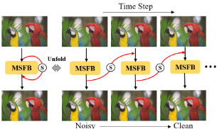
Figure 1: Schematic diagram of selective multi-scale feedback mechanism and dual learning. (a) The principle of our MSFB scheme unfolding in time. The "S" on the feedback loop represents the selective mechanism. (b) Dual regression training scheme, which contains a primal regression task for denoising and a dual regression task to project clean images back to noisy images.
It is difficult for a single-stage supervised image denoising network to find the best mapping from noise to clean in the infinite solution space. The two-stage methods for image denoising include noise estimation and removal. But the twostep structure increases network complexity and accumulates errors inevitably. In network optimization, most end-to-end networks strive to minimize the difference between clean labels and the predicted images. However, it is challenging to predict complex degradation with only one-step supervision in the clean domain. Due to the lack of noise-free labels, many unpaired real-world noise images that are easily available cannot participate in general fully-supervised training, which limits network performance and adaptability to real noise. Networks that rely excessively on high-quality images are likely to overfit the synthetic noise. Dual learning [He et al.2016] uses closed-loop dual tasks to optimize the network. Adding additional supervision in the noise domain can make the network more robust to various noise. Some methods used for high-level tasks such as CycleGAN [Zhu et al.2017] and DualGAN [Yi et al.2017] discard a large number of task-independent image details, so they cannot be directly transferred to the image-to-image denoising task.
We design a novel multi-scale selective feedback network (MSFN) with the dual loss for real image denoising based on the above discussion. The commonly used one-step prediction is replaced by a multi-level iterative prediction, which guides image restoration from coarse to fine adaptively. As shown in Fig. 1(a), the multi-scale selective feedback block (MSFB) is unfolded in time. We count each iteration into the total loss to ensure that the hidden unit to be fed back contains reliable high-level functions. Using too many high-level semantic features will overwhelm the original low-level information. The selective feedback mechanism is proposed to analyze principal feature components. We reduce feature redundancy through principal component analysis (PCA), which captures the most representative information. The multiscale selective block (MSB) integrates multi-scale features for changing receptive fields dynamically. The step-by-step learning strategy is proven to be more suitable for fitting various real-world degradations accurately.
As shown in Fig. 1(b), we decompose the noise removal task into closed-loop dual tasks. The primary task predicts noise-free images ˆY from the noise image X, and the dual regression task restores the original noise image ˆX from ˆY reversely. We introduce a weighting mechanism to design dual loss to guide network optimization. The closed-loop dualdomain supervision can reduce the solution space and alleviate the model's excessive dependence on clean images. For paired data, there is a complete dual loss. For unpaired data, the loss function only includes supervision in the noise domain. Unpaired real-world images can directly participate in network training. We can expand diversified noise types in the training set freely and effectively, which reduces the risk of network overfitting to a specific noise level. In summary, our contribution has the following three points:
- The proposed MSFN allows shallow layers to access valuable information from the following deep layers selectively. Combining bottom-up multi-level intermediate supervision and the top-down feedback mechanism can remove complex noise from coarse to fine.
- We design a dual weighted loss combining clean-tonoisy and noisy-to-clean tasks. The closed-loop multidomain supervision is easier to learn the best mapping in an infinite solution space. Dual loss can perform endto-end training on unpaired data, which has better generalization and adaptability to real-world noise images.
- Dual loss and feedback learning strategies can be adapted to different denoising tasks, including complex degraded and unsupervised images. Extensive experiments prove that our proposed network achieved the best denoising performance in multiple synthetic noise images and paired or unpaired real-world noise images.
2 ProposedMethod
2.1 Overall Network Architecture
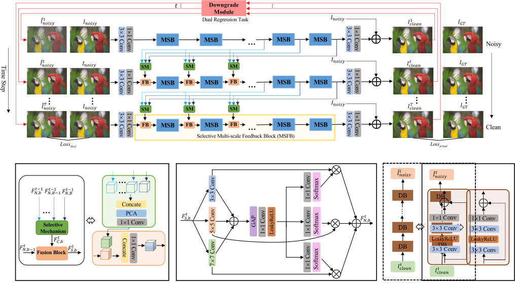
The feedback network contains two essential elements: iterability and the reverse connection from deep to shallow. As shown in Fig. 3(a), we designed the multi-scale selection block (MSB) to extract features with multiple receptive fields and the selective feedback module (SFM) to capture valuable deep features to assist shallow denoising adaptively. Our proposed multi-scale selective feedback network (MSFN) can be expanded into an independent convolutional neural network with T iterations. We train two regression tasks in the noise domain and the clean domain jointly at each time step.
We define the input image of each iteration in MSFN as Inoisy. Firstly, we use two convolutional layers with convolution kernel sizes of 3×3 and 1×1 to extract the initial shallow feature F t N,0 , which can be expressed as:
where MSFE(·) represents the shallow feature extraction (SFE) function. After that, the initial feature is transferred to the recurrent structure that contains the stacked MSBs. The MSB fuses multi-scale information by changing receptive fields and selects useful features for image denoising adaptively and dynamically. The MSB is detailed in Section 2.3.
As shown in Fig. 3(a), when t = 0, there is no high-level information fed back from the previous step. The feed-forward shallow layers access useful information from the following layers when 0 < t ≤ T . Assuming that the number of stacked MSBs in the feed-forward network is B, then the feature F t N,B output by the last MSB in each time step is expressed as:
where MMSFB(·) is the function that combines B MSBs and M SFMs. The principal components of high-level features from the previous time step are fused with the shallow features adaptively. Dynamically aggregated context allows topdown and bottom-up real-time knowledge exchange.
At the end of each time step, the reconstruction function is defined as MR(·), which includes two convolutional layers and a residual skip connection. The final output of our denoised image in the t -th iteration can be expressed as:
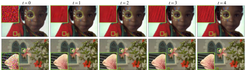
We visualize the iterative restoration process in Fig. 2. The structural edges and textures are refined step by step, proving that the feedback hierarchical learning strategy can reconstruct high-quality details from coarse to fine.
In each time step, we design a dual regression task to constrain the pixel prediction further. As shown by the red arrows Time Step Time Step in Fig. 3(a), the reverse degradation model (DM) generates noisy correspondences to the predicted images at each time step. As shown in Fig. 3(d), the DM is composed of stacked degradation blocks (DB). The DM function MDM(·) remaps the clean image to the image ˆ Inoisy in the noise domain. The degradation process of the t-th iteration is defined as:
where MDB(·) represents the DB, and the convolution kernel sizes of the convolutional layer are 3×3, 3×3, and 1×1, respectively, and the activation layer LeakyReLU follows the first convolutional layer. We set k = 8 and the DM output degraded noisy image predicted by the dual regression task.
In the primary regression, we get T predicted noise-free images. Simultaneously, other T noise images are restored by dual regression tasks. We design a novel asymmetric dual loss to optimize the dual model jointly. As shown in Fig. 3(a), the dual loss is weighted by Lossprimal in the clean domain and Lossdual in the noisy domain, which can be defined as:
where q represents all the learnable parameter in MSFN. IGT stands for ground truth (GT). I t clean and ˆ I t noisy represent the predicted clean image and predicted noisy image in the t-th step, respectively. The adaptive weighting with l1 and l2 can guide the task optimization with attention. For unpaired realworld noisy images without clean labels, l1 is set to 0.
2.2 Selective FeedbackModule
Integration of all unprocessed high-level feedback will bring information redundancy, which will overwhelm the original shallow features. We improved the multi-level feedback and showed the internal implementation details in Fig 3(b).
Firstly, we use the selective mechanism (SM) to analyze the principal feature components. The correlated highdimensional features are transformed into mutually independent low-dimensional information. We perform principal component analysis (PCA) on the fused features. We decompose the singular value of the feature X ∈ R(h×w)×c as:
where ˆX ∈ R(h×w)×c/r . For the t-th iteration, the selected potential clean feature F t C,b to be fed back is expressed as:
where F t-1 N,b , · · · ,F t-1 N,B-1 , F t-1 N,B is the high-level feedback features from different depths. The number of feedback branches is defined as m, ie.m=B-b. These high-level components are concatnated into a whole in the channel direction.
For the b-th MSB, we fuse the feedback feature F t C,b and feed-forward feature F t N,b-1 by the fusion block (FB) as:
where the F t S,b is the refined low-level features.
| Method | Kodak24 | BSD68 | Urban100 | |||||||||
|---|---|---|---|---|---|---|---|---|---|---|---|---|
| 10 | 30 | 50 | 70 | 10 | 30 | 50 | 70 | 10 | 30 | 50 | 70 | |
| CBM3D [Dabov et al.2007] | 36.57 | 30.89 | 28.63 | 27.27 | 35.91 | 29.73 | 27.38 | 26.00 | 36.00 | 30.36 | 27.94 | 26.31 |
| TNRD [Chen and Pock2017] | 34.33 | 28.83 | 27.17 | 24.94 | 33.36 | 27.64 | 25.96 | 23.83 | 33.60 | 27.40 | 25.52 | 22.63 |
| RED [Mao et al.2016] | 34.91 | 29.71 | 27.62 | 26.36 | 33.89 | 28.46 | 26.35 | 25.09 | 34.59 | 29.02 | 26.40 | 24.74 |
| DnCNN [Zhang et al.2017a] | 36.98 | 31.39 | 29.16 | 27.64 | 36.31 | 30.40 | 28.01 | 26.56 | 36.21 | 30.28 | 28.16 | 26.17 |
| MemNet [Tai et al.2017] | N/A | 29.67 | 27.65 | 26.40 | N/A | 28.39 | 26.33 | 25.08 | N/A | 28.93 | 26.53 | 24.93 |
| IRCNN [Zhang et al.2017b] | 36.70 | 31.24 | 28.93 | N/A | 36.06 | 30.22 | 27.86 | N/A | 35.81 | 30.28 | 27.69 | N/A |
| FFDNet [Zhang et al.2017c] | 36.81 | 31.39 | 29.10 | 27.68 | 36.14 | 30.31 | 27.96 | 26.53 | 35.77 | 30.53 | 28.05 | 26.39 |
| RNAN [Zhang et al.2019] | 37.24 | 31.86 | 29.58 | 28.16 | 36.43 | 30.63 | 28.27 | 26.83 | 36.59 | 31.50 | 29.08 | 27.45 |
| MSFN (Ours) | 37.49 | 32.08 | 29.81 | 28.38 | 36.66 | 30.84 | 28.52 | 27.17 | 36.95 | 31.93 | 29.63 | 27.98 |
2.3 Multi-scale Selective Block
The changing receptive field brings more contextual information. We design a selective mechanism to adjust the selfattention of the multi-scale feature. As shown in Fig 3(c), the MSB extracts features through three convolutional layers with different convolution kernels and aggregates multiple branches according to the significance dynamically.
Specifically, the MSB contains three branches with convolution kernels of 3×3, 5×5, and 7×7. For the b-th MSB, the multi-scale information of feature F t S,b is described as:
where f3, f5, and f7 are the outputs of each path.
We use the global average pooling and LeakyReLU activation function to squeeze and excite the fused feature. The output global feature descriptor F t f ,b is:
The self-attention mapping (SAM) recalibrates the correlation of each branch. The fuction MSAM includes convolution and the softmax regression to map the descriptor as:
where a3, a5, and a7 are the attention vectors. The valuable and representative information at each scale is remapped as:
The multi-scale features are selected and gathered for critical cross-layer and cross-scale information interaction.
3 Experiments
3.1 Datasets
Synthetic Noisy Images. The DIV2K [Timofte et al.2017] and Flickr2K [Lim et al.2017] datasets are used to generate synthetic noise images. There are 3100 images used for training and 350 images for verification. We add white Gaussian noise with levels of s = 10, 30, 50, 70 for paired data. We will evaluate the trained network on common benchmark datasets, including BSD68, Kodak24, and Urban100.
Real Noisy Images. The real-world noise images come from the SIDD [Abdelhamed and Lin2018]. Specifically, SIDD includes 10 static scenes of 5 smartphones with different shooting pipeline settings, which are under different lighting conditions. The SIDD-Medium dataset that we used consists of 320 image pairs. We additionally use three other public real-world noise data sets for model testing, including PolyU [Xu et al.2018a], Nam [Nam et al.2016], and Darmstadt Noise Dataset (DND) [Plotz and Roth2017]. The unpaired data used for adaptive training come from the SIDDFull dataset 1 . To verify the proposed noise domain supervision effectiveness, we select 200 images that do not overlap with the original training set. It should be noted that unpaired data do not use clean reference images in the training process.
1 https://www.eecs.yorku.ca/ kamel/sidd/dataset.php
| Method | SIDD | DND |
|---|---|---|
| DnCNN-B [Zhang et al.2017a] | 23.66 / 0.583 | 32.43 / 0.790 |
| FFDNet+ [Zhang et al.2017c] | - / - | 37.61 / 0.942 |
| CBDNet [Guo et al.2019] | 33.28 / 0.868 | 38.06 / 0.942 |
| RIDNet [Anwar and Barnes2019] | 38.71 / 0.914 | 39.26 / 0.953 |
| VDN [Yue et al.2019] | 39.23 / 0.955 | 39.38 / 0.952 |
| AINDNet [Kim et al.2020] | 39.15 / 0.955 | 39.53 / 0.956 |
| MIRNet [Zamir et al.2020] | 39.72 / 0.959 | 39.88 / 0.956 |
| MSFN (Ours) | 39.98 / 0.973 | 40.01/ 0.963 |
| MSFN-U (Ours) | 40.12 / 0.974 | 40.12/ 0.965 |
| Method | PolyU | Nam |
|---|---|---|
| DnCNN-B [Zhang et al.2017a] | 34.68 / 0.874 | 34.95 / 0.885 |
| NC [Lebrun and Colom2015] | 36.84 / 0.936 | 37.69 / 0.952 |
| MCWNNM [Xu et al.2017] | 37.72 / 0.945 | 37.84 / 0.956 |
| RDN [Zhang et al.2020] | 37.94 / 0.946 | 38.16 / 0.956 |
| FFDNet+ [Zhang et al.2017c] | 38.17 / 0.951 | 38.81 / 0.957 |
| TWSC [Xu et al.2018b] | 38.68 / 0.958 | 38.96 / 0.962 |
| CBDNet [Guo et al.2019] | 38.74 / 0.961 | 39.08 / 0.969 |
| RIDNet [Anwar and Barnes2019] | 38.86 / 0.962 | 39.20 / 0.973 |
| VDN [Yue et al.2019] | 39.04 / 0.965 | 39.68 / 0.976 |
| MSFN (Ours) | 40.68 / 0.977 | 40.81 / 0.985 |
| MSFN-U (Ours) | 40.79 / 0.978 | 40.95 / 0.987 |
3.2 Implementation Details
The MSFN has 30 MSBs and 4 SFMs in the sub-network at each time step. We set unfolded time steps as T = 4. We set up a multiple-to-multiple feedback connection (m= 4). The reduction factor r in PCA is 16, and the DM has 8 DBs. The weighting coefficients in dual loss are {l1 = 0.9,l2 = 0.1}. In the synthetic datasets, 16 patches cropped to 96×96 form a training batch, while in the real-world datasets, the setting is 32 patches that cropped to 128×128. The number of feature channels is 64, except for the input and output layer. We set the initial learning rate as 1×10⁻⁴ and use the ADAM optimization method with parameter {b1 = 0.9, b2 = 0.999, e = 10-8}. All models are implemented in PyTorch and trained on NVIDIA GeForce RTX 2080 Ti GPU.
3.3 Comparisons with Other Methods
We perform qualitative and quantitative comparisons on the standard benchmarks. The metrics are peak signal-to-noise ratio (PSNR) and structural similarity index metric (SSIM).
Quantitative Comparison
Synthetic Noise. We evaluate different methods including CBM3D [Dabov et al.2007], TNRD [Chen and Pock2017], RED [Mao et al.2016], DnCNN [Zhang et al.2017a], MemNet [Tai et al.2017], IRCNN [Zhang et al.2017b], FFDNet [Zhang et al.2017c], and RNAN [Zhang et al.2019]. The quantitative and qualitative comparison results of all methods on the three benchmark data sets of Kodak24, BSD68, and Urban100 are shown in Tab. 1. The proposed MSFN achieves the best performance on all noise levels and all benchmark datasets, which increases the highest PSNR by more than 0.2 dB. Our method shows superiority on severely degraded images with a noise level of s = 70. On the Urban100 dataset, MSFN increases the highest PSNR from 27.45 dB to 27.98 dB. The iterative feedback mechanism reduces the difficulty of training and accelerates convergence step by step.
Real-World Noise. We compare the performance of nine real-world denoising methods on PolyU and Nam, and seven methods on SIDD and DND, including DnCNN-B [Zhang et al.2017a], Noise Clinic (NC) [Lebrun and Colom2015], MCWNNM [Xu et al.2017], RDN [Zhang et al.2020], FFDNet+ [Zhang et al.2017c], TWSC [Xu et al.2018b], CBDNet [Guo et al.2019], RIDNet [Anwar and Barnes2019], VDN [Yue et al.2019], AINDNet [Kim et al.2020], and MIRNet [Zamir et al.2020]. The dual loss can supervise images in the noise domain independently so that we can add unpaired data for training. As shown in Tab. 2 and Tab. 3, the proposed MSFN shows significant superiority and good generalization on the real-world images denoising. Compared with the latest MIRNet, our network achieved a performance gain of 0.26 dB on SIDD and 0.14 dB on DND. The performance on PolyU and Nam also exceeds other methods by a large margin, improving at least 1.64 dB and 1.13 dB, respectively. The network fine-tuned by 200 unpaired noise images is defined as MSFN-U, which improves the model performance on the 4 datasets by at least 0.11 dB. The MSFN based on dual loss can make full use of unpaired training data and does not rely on noise-free labels excessively. Experiments prove that training with paired and unpaired data is optimal.
| Method | Feedback Mechanism | Dual Regression | PSNR (dB) / SSIM |
|---|---|---|---|
| A B C D (Ours) | ✓ ✓ | ✓ ✓ | 37.97 / 0.948 38.63 / 0.949 39.37 / 0.952 40.01 / 0.963 |
| Weight | |||||||
|---|---|---|---|---|---|---|---|
| l1 | 0 | 0.1 | 0.3 | 0.5 | 0.7 | 0.9 | 1 |
| l2 | 1 | 0.9 | 0.7 | 0.5 | 0.3 | 0.1 | 0 |
| PSNR (dB) | 25.86 | 26.75 | 27.83 | 28.61 | 29.38 | 29.81 | 29.57 |
Visual Comparison
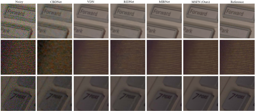
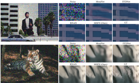
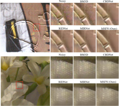
We compare denoising results with a noise level of s = 50 on BSD68 in Fig. 5. The result of MSFN is the closest to the ground truth compared with other methods. The MemNet, FFDNet, and RNAN deform and blur the structural texture, which causes distortion and loss of details. The image restored by our MSFN can retain more original structures while removing noise. The visual comparison on SIDD benchmark datasets is shown in Fig. 4. Recovering contaminated characters clearly and accurately is difficult for previous methods. The structural textures are excessively smoothed and appear artifacts or chromatic aberration after processing by previous RIDNet and MIRNet. Our MSFN shows superiority in preserving structural content and fine texture details, resulting in pleasantly clear images. As shown in Fig. 6, our MSFN has better adaptability to the unevenly distributed real-world noise. Compared with reference images, our method effectively removes noise and achieves reliable results.
3.4 Ablation Study
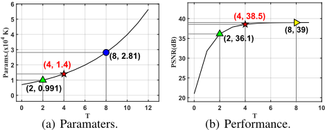
Time Steps. Fig. 7(a) and Fig. 7(b) show the response curves of model complexity and performance to T, respectively. We take T = {2,4,8} and use green, red, and blue markers to mark the corresponding points in the figure. As the iteration proceeds, the amount of model learnable parameters increases in a non-linear exponential trend, and the PSNR also increases. When T further increases to greater than 4, the growth of PSNR slows down. When T > 8, the denoising performance (39 dB) hardly improves, along with the rapidly increasing parameter quantity. Therefore, we set T = 4 to balance model performance and computational complexity.
Component Analysis. We analyze the performance of different network component combinations on the DND. As shown in Tab. 4, method A is a baseline with no feedback and no duality. Methods B and C introduce feedback mechanisms and dual loss, respectively. The feedback mechanism refines the high-level information to guide low-level features and increases 1.4 dB compared to baseline. The dual supervision narrows the solution space by additional constraints and obtains a performance gain of 0.66dB. The method D combining feedback and dual regression strategies gains the best denoising ability as high as 40.01 dB. Eq. (6) introduces two hyper-parameters l1 and l2 to adjust the weights of primary and dual regression losses. We set different weights during training and tested it on Kodak24 with s = 70. As shown in Tab. 5, when {l1 = 0, l2 = 1}, only supervising the noise domain results in a poor performance. Relaxed constraints lead to ill-posed uncertain mapping. Therefore, the increase of l1 achieves a significant performance gain. When {l1 = 0.9,l2 = 0.1}, the learned model obtains the highest PSNR (29.81 dB).After canceling the noise fitting loss (l2 = 0), the PSNR decreases by 0.24dB, which proves the necessity of the dual regression task.
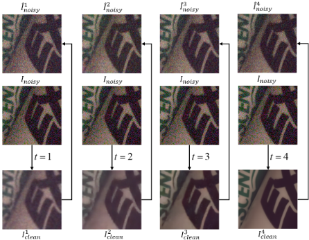
Unpaired Supervision. The denoising of unpaired data is visualized in Fig 8. The feed-forward noise image Inoisy outputs the predicted image I t clean and then degenerates to the reconstructed ˆ Inoisy in the noise domain step by step. As shown in Fig 8, unpaired real noisy images can obtain reliable restoration only through the noise domain supervision. The MSFN outputs refined noise-free images from coarse to fine and refits the original noise as much as possible. The unpaired real-world noise images can be used for model training and fine-tuning. The effective expansion of real-world images further increases the model adaptability. It can alleviate the model's excessive dependence on labels and noise overfitting.
4 Conclusion
In this paper, we propose a novel network for real-world image denoising, called multi-scale selective feedback network (MSFN) with dual loss. By propagating the principal components of the high-level hierarchical features to the shallow layers, the selective feedback module (SFM) enriches the early representation learning effectively. Iterative multi-scale feature reusing in multiple time steps is conducive to fitting complex degradation from coarse to fine. The proposed dual loss method provides a more strict closed-loop supervision on both the noise domain and the clean domain for paired and unpaired data. The comprehensively experimental results prove that our method is superior to the state-of-the-art methods and has better applicability to real-world data.
Acknowledgments
This work is partially supported by the NSFC fund (61831014), in part by the Shenzhen Science and Technology Project under Grant (ZDYBH201900000002, JCYJ20180508152042002, GGFW2017040714161462).
@inproceedings{ijcai2021p101,
  title     = {Multi-Scale Selective Feedback Network with Dual Loss for Real Image Denoising},
  author    = {Hu, Xiaowan and Cai, Yuanhao and Liu, Zhihong and Wang, Haoqian and Zhang, Yulun},
  booktitle = {Proceedings of the Thirtieth International Joint Conference on
               Artificial Intelligence, {IJCAI-21}},
  publisher = {International Joint Conferences on Artificial Intelligence Organization},
  editor    = {Zhi-Hua Zhou},
  pages     = {729--735},
  year      = {2021},
  month     = {8},
  note      = {Main Track},
  doi       = {10.24963/ijcai.2021/101},
  url       = {https://doi.org/10.24963/ijcai.2021/101},
}
TY - CPAPER TI - Multi-Scale Selective Feedback Network with Dual Loss for Real Image Denoising AU - Hu, Xiaowan AU - Cai, Yuanhao AU - Liu, Zhihong AU - Wang, Haoqian AU - Zhang, Yulun T2 - Proceedings of the Thirtieth International Joint Conference on Artificial Intelligence, IJCAI-21 PB - International Joint Conferences on Artificial Intelligence Organization PY - 2021 SP - 729 EP - 735 DO - 10.24963/ijcai.2021/101 UR - https://doi.org/10.24963/ijcai.2021/101 ER -Copied
Machine-readable versions of this paper, for tools and AI agents:





