Causal Discovery with Multi-Domain LiNGAM for Latent Factors

1 Introduction

Learning causal relationships from observed data, termed as causal discovery, has been developed rapidly over the past decades [Pearl, 2009; Spirtes and Zhang, 2016; Peters et al., 2017]. In many scenarios, including sociology, psychology, and educational research, the underlying causal relations are usually embedded between latent variables (or factors) that cannot be directly measured, e.g., anxiety, depression, or coping, etc [Silva et al., 2006; Bartholomew et al., 2008], in which scientists are often interested.

Some approaches have been developed to identify the causal structure among latent factors, which can be categorized into covariance-based and non-Gaussianity-based ones. Covariance-based methods employ the covariance structure of data alone, e.g., BuildPureClusters algorithm [Silva et al., 2006], or FindOneFactorClusters algorithm [Kummerfeld and Ramsey, 2016], to ascertain how many latent factors as well as the structure of latent factors. However, these algorithms can only output structures up to the Markov equivalence class for latent factors. Non-Gaussianity-based methods address this indistinguishable identification problem by taking the best of the non-Gaussianity of data. Specifically, Shimizu et al. [2009] leveraged non-Gaussianity and firstly achieved identifying a unique causal structure between latent factors based on the Linear, Non-Gaussian, Acyclic Models (LiNGAM) [Shimizu et al., 2006]. They transformed the problem into the Noisy Independent Component Analysis (NICA). Recently, to avoid the local optima of the NICA, Cai et al. [2019] designed the so-called Triad constraints and Xie et al. [2020] developed the GIN condition. They both proposed a two-phase method to learn the structure or causal orderings among latent factors.

It is noteworthy that the above-mentioned methods all focus on the data which are originated from the same domain, i.e., single-domain data. However, in many real-world applications, data are often collected under distinct conditions. They may be originated from different domains, resulting in distinct distributions and/or various causal effects. For instance, in neuroinformatics, functional Magnetic Resonance Imaging (fMRI) signals are frequently extracted from multiple subjects or over time [Smith et al., 2011]; in biology, a particular disease is measured by distinct medical equipment [Dhir and Lee, 2020], etc. Existing methods to handle multi-domain data in causal discovery are flourishing, e.g., Danks et al. [2009], Tillman and Spirtes [2011], Ghassami et al. [2018], Kocaoglu et al. [2019], Dhir and Lee [2020], Huang et al. [2020], Jaber et al. [2020], etc. Though there are some methods to handle multi-domain data that allow the existence of latent variables or confounders, no such method is yet proposed in the literature when learning the causal structure among latent factors with only observed data, to our best knowledge. Thus, it is desirable to perform causal discovery from multi-domain data to uncover the structure among latent factors.

When considering multi-domain instead of single-domain data in latent factor models, there may exist different causal structures among latent factors or with different causal effects in different domains. An important question then naturally raises, i.e., how to guarantee that factors in different domains are represented by the same factors of interest so that the underlying structure among latent factors of interest is uncovered. A solution may be to naively concatenate the multi-domain observed data, such that the multi-domain model can be regarded as a single-domain latent factor model. However, it may cause serious bias in estimating the causal structure among latent factors of interest [Shimizu, 2012]. In this paper, we propose Multi-Domain Linear Non-Gaussian Acyclic Models for LAtent Factors (MD-LiNA) to represent the causal mechanism of latent factors, which tackles not only single-domain data but multi-domain ones. In addition, we propose an integrated two-phase approach to uniquely identify the underlying causal structure among latent factors (of interest). In particular, in the first phase, we locate the latent factors and estimate the factor loading matrix (relating the observed variables to its latent factors) for all domains, leveraging the ideas from Triad constraints and factor analysis [Cai et al., 2019; Reilly and O'Brien, 1996]. In the second phase, we derive a score function to characterize the independence relations between external variables, and interestingly, we unify this function to characterize the dependence relations between latent factors from different domains and latent factors of interest. Then such unified function is enforced with acyclicity, sparsity, and elastic net constraints, with which our task is formulated as a purely continuous optimization problem. The method is (locally) consistent to produce feasible solutions.

Our contributions are mainly three-folded:

• This is the first effort to study the causal discovery problem of identifying causal structures between latent factors for multi-domain observed data.
• We propose an MD-LiNA model, which is a causal representation for both single and multi-domain data in latent factor models and offers a deep interpretation of dependencies between observed variables across domains, and show its identifiability results.
• We propose an integrated two-phase approach to uniquely estimate the underlying causal structure among latent factors, which simultaneously identifies causal directions and effects. It is capable of handling cases when the sample size is small or the latent factors are highly correlated. And the local consistency is also provided.

2 ProblemFormalization

Suppose we have data from M domains. Let x(m) and f (m) (m = 1, ...,M) be the random vectors that collect pm observed variables and qm latent factors in domain m, respectively. The total number of observed variables for all domains is p = ∑Mm=1 pm while that of latent factors is q = ∑Mm=1 qm. In this study, we focus on linear models,

1 These waved lines are used to emphasize the common space and they can be simply replaced by directed edges.

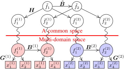
where ε(m) , and e(m) are random vectors that collect external influences, and errors, respectively, and they are independent with each other. B(m) is a matrix that collects causal effects b(m) ij between f (m) i and f (m) j , while G(m) collects factor loadings g(m) ij between f (m) j and x(m) i . f (m) i is assumed to have zero means and unit variances. Note that in a specific domain m, data are generated with the same b(m) ij and g(m) ij . ε(m) i and e(m) i are sampled independently from the identical distributions. In different domains, B(m1) (G(m1) ) and B(m2) (G(m2) ) may be different, but they have a shared causal structure.

Thereafter, we encounter two problems: how to integrate the multi-domain data effectively ; and how to guarantee factors f in different domains are represented by the same concepts (factors) of interest, with which we identify the underlying causal structure among latent factors of interest. To address the first problem, we leverage an idea of simple coding representation [Shimodaira, 2016], i.e., an observation is represented as an augmented one with p dimensions, where only pm dimensions come from the original domain while the other (p - pm) dimensions are padded with zeros. Any augmented data are expressed with a bar, e.g., ¯x and ¯ f . With such representations, we obtain,

where ¯B = Diag(B(1) , ...,B(M) ), ¯ ε and ¯ e are independent, and ¯G = Diag(G(1) , ...,G(M) ). A detailed explanation is presented in Supplementary Materials A (SM A). To address the second problem, we introduce factors of interest ˜ f , which are embedded as different concepts with causal relations. As depicted in Figure 1, suppose ¯ f are linearly generated by ˜ f ,

where H ∈ Rqט q (˜ q ≤ q) is a transformation matrix, and ˜ q is the number of ˜ f. The whole model is defined as follows.

Definition 1 (Multi-Domain LiNGAM for LAtent Factors (MD-LiNA)). An MD-LiNA model satisfies the following assumptions:

• A1. f (m) are generated linearly from a Directed Acyclic Graph (DAG) with non-Gaussian distributed external variables ε(m) , as in Eq.(1);
• A2. x(m) are generated linearly from f (m) plus Gaussian distributed errors e(m) , as in Eq.(1);
• A3. Each fi has at least 2 pure measurement variables 2 ;
• A4. Each ¯ fi (m) is linearly generated by only one latent in ˜ f and each ˜ fi generates at least one latent in ¯ f, as in Eq.(3).

Note that assumption A4 implies that each row of H has only one non-zero element and each column has at least one non-zero element. It is reasonable since it is equal to the most interpretable structure in factor analysis. More plausibility of assumptions is discussed in SM B.

Once given multi-domain data, our goal is to estimate ¯G and ˜B, where ˜B is a matrix that collects causal effects between shared latent factors of interest ˜ f. ˜B reflects the underlying causal structure shared by different B(m) . If there is only one single domain in the data, one just needs to estimate ¯G = G(1) and B(1) , where assumption A4 can be neglected and our model is simply called LiNGAM for LAtent Factors (LiNA). For simplicity, we use the measurement model to relate the structure from x(m) to f (m) while the structure model to record the causal relations among ˜ f or f (m) [Silva et al., 2006].

3 Model Identification

We state our identifiability results here. Note that the identifiability of LiNA has been provided by Shimizu et al. [2009], but with the assumption that each latent factor has at least 3 pure measurement variables. Below we show this identifiability can be strengthened to 2 pure measurement variables for each factor inspired by Triad constraints [Cai et al., 2019].

Lemma 1. Assume that the input data X strictly follow the LiNA model. Then the factor loading matrix G is identifiable up to permutation and scaling of columns and the causal effects matrix B is fully identifiable.

The proof is in SM C. It relies on the corollary that Triad constraints also hold for our models, which helps find pure measurement variables and achieve LiNA's identifiability. Next, we show the identifiability of MD-LiNA in Theorem 1.

Theorem 1. Assume that the input multi-domain data X with X(m) of domain m, strictly follow the MD-LiNA model. Then the underlying factor loading matrix ¯G is identifiable up to permutation and scaling of columns and the causal effects matrix ˜B is fully identifiable.

We give a sketch of the proof below. For complete proofs of all theoretical results, please see SMC.

2 Pure measurement variables are those which have only one single latent factor parent [Silva et al., 2006].

Proof Sketch. Firstly in Eq.(2) and due to Lemma 1, ¯G is identifiable up to permutation and scaling of columns, since we estimate one measurement model for all domains simultaneously (mentioned in Section 4). Furthermore, combining Eqs.(2) and (3), we obtain ˜ f = ˜B ˜ f + ˜ ε, where ˜B = (HT H)-1HT ¯BH ∈ R˜ qט q and ˜ ε = (HT H)-1HT ¯ ε ∈ R˜ q . Note that the inverse matrix of HT H always exists since H is full column rank due to the assumption A4. To prove ˜B is identifiable, we have to additionally ensure ˜B can be permuted to a strictly lower triangular matrix and ˜ ε are independent with each other. Fortunately, due to assumption A1, ˜B satisfies the condition. Due to assumption A4, by virtue of the independence between ¯ ε, its non-Gaussianity and the Darmois-Skitovich theorem [Kagan et al., 1973], ˜ ε are also independent with each other. Thus, ˜B is fully identifiable, which implies the theorem is proved.

4 Model Estimation

We exhibit a two-phase framework (measurement-model and structure-model phases) to estimate causal structures under latent factors in Algorithm 1, and provide its consistency.

4.1 MD-LiNAAlgorithm

To learn measurement models, we have several approaches. Firstly, we can use the Confirmatory Factor Analysis (CFA) [Reilly and O'Brien, 1996], after employing Triad 3 to yield the structure between latent factors f (m) and observed variables x(m) [Cai et al., 2019]. Secondly, more exploratory approaches are advocated, e.g., Exploratory Structural Equation Modeling (ESEM) [Asparouhov and Muth´en, 2009], which enables us to use fewer restrictions on estimating factor loadings. Please see SM D for details. In our paper, we take the first approach, as illustrated in lines 1 to 3 of Algorithm 1, but we can use the second one as well in our framework.

To learn structure models, we introduce the log-likelihood function of LiNA, then unify it to MD-LiNA. For brevity, we omit the superscripts of all notations for LiNA. The loglikelihood function of LiNA is derived by characterizing the independence relations between ε from NICA models,

where ‖x‖2Σ-1 = xT Σ-1x, X(t) is the tth column (observation) of data X. ˆG is the estimate of G. ˜ˆGT = ( ˆGT ˆG)-1 ˆGT relates to ˆG and gi is the ith column of ˜ˆG. The inverse matrix of ˆGT ˆG always exists due to assumption A3. bi denotes the ith column of BT . n is the sample size. C is a constant and ˆ pi is their corresponding density function, which is specified to be Laplace distribution in estimation. Please see SM E.1 for detailed derivations.

3 Triad constraints help locate latent factors and learn the causal structure between them, but they focus on single-domain data.

Algorithm 1 MD-LiNA Algorithm

Input: Data X(1) , ...,X(M) ; M.

Output: Factor loadings ¯G (G); effects matrix ˜B (B).

Phase I: Measurement models

• 1: Find the number of latent factors qm and locate latent factors for each domain m by Triad constraints;
• 2: Get augmented data ¯X = Diag(X(1) , ...,X(M) ) and estimate ¯G by CFA;
• 3: Estimate ¯ f .= ( ¯GT ¯G)-1 ¯GT ¯X; Phase II: Structure models
• 4: if M > 1 then
• 5: Optimize Eq.(7) iteratively for H and ˜B until convergence using QPM (or ALM);
• 6: Update ˜B with regard toH;
• 7: else
• 8: Optimize Eq.(5) to get B with QPM (or ALM);
• 9: end if
• 10: return ¯G and ˜B (M > 1 ); or G= ¯G and B (M = 1).

Further, to strengthen the learning power in different cases, e.g., with small sample sizes or multicollinearity problem, we render B to satisfy an acyclicity constraint, adaptive ℓ1 as well as ℓ2 regularizations [Zheng et al., 2018; Hyv¨arinen et al., 2010; Zou and Hastie, 2005],

h(B) = tr(eB◦B ) - q is the needed acyclicity constraint. ◦ is the Hadamard product, and eB is the matrix exponential of B. ‖B‖1∗ = ∑qi=1 ∑qj=1 |bij|/|ˆbij| represents the sparsity constraint where ˆbij in ˆB is estimated by maximizing L(B, ˆG). ‖B‖2 is the ℓ2 regularization. λ1 and λ2 are regularization parameters. This optimization function facilitates the simultaneous estimation of causal directions and effects between latent factors, without additional steps of permutation and rescaling, as required in Shimizu et al. [2009].

Thus, with estimated ˆG, we leverage the Quadratic Penalty Method (QPM) (or Augmented Lagrangian Method, ALM) to optimize B, transforming Eq. (5) into an unconstrained one,

in which S(B) = F(B, ˆG) + ρ2 h(B)2 is the quadratic penalty function. ρ is a regularization parameter. (For ALM, S(B) = F(B, ˆG) + ρ2 h(B)2 + αh(B), where α is a Lagrange multiplier.) Then Eq.(6) is solved by L-BFGS-B [Zhu et al., 1997]. In case of avoiding numerical false discoveries from estimation, edges whose estimated effects are under a small threshold ϵ are ruled out [Zheng et al., 2018].

Next, we show how Eq.(5) is unified to handle multidomain cases (M > 1). Firstly, all X(m) are projected into ¯X in a single common space so that ¯ f are estimated. We then introduce the dependence relations between ˜ f and ¯ f in Eq.(5), i.e., reconstruction errors E(H) and an adaptive

E(H) = ‖ ¯ f -H ˜ f‖2 = ‖ ¯ f - PH ¯ f‖2 , and λ3 is a regularization parameter. PH = H(HT H)-1HT is a projection matrix onto the column space of H. F( ˜B,H) is the loglikelihood of MD-LiNA,

where ˜¯GT = ( ¯GT ¯G)-1 ¯GT , ˜ˆHT = (HT H)-1HT , the inverse matrices of HT H and ¯GT ¯G always exist due to assumptions A3 and A4. hi is the ith column of ˜ˆH. ˜bi denotes the ith column of ˜BT . See SM E.2 for detailed derivations.

We iteratively optimize H and ˜B using QPM (or ALM) until convergence. Specifically for QPM, i) to optimize H, we find its descent direction to derive the next iteration for a given ˜B. Since there is no constraints for H, it is an unconstrained problem. ii) to optimize ˜B, we compute its descent direction for the next iteration given H, and update the penalty parameter ρ until the acyclicity constraint h( ˜B) = 0 is satisfied. Finally, we repeat steps i) and ii) until H and ˜B are convergent. With H, we can link the factors from multiple domains with high weights together to symbolize the same concepts so that we can decide which factors from different domains are represented by which factors of interest. Specifically, for ˜ fi, those factors ¯ f from different domains with the largest weights are considered to be represented by this ˜ fi, where ˜ fi can also be named according to its corresponding observed measurement variables. Then according to these represented factors ¯ f for each ˜ fi, we obtain the causal ordering among ˜ f, with which ˜B can be updated. For the computational complexity, please see SM F.

4.2 Consistency Proofs

Here we prove that our methods could provide locally consistent estimators for MD-LiNA, including LiNA.

Theorem 2. Assume the input single-domain data X strictly follow the LiNA model. Given that the sample size n, the number of observed variables p and the penalty coefficient ρ satisfy n, p, ρ → ∞, then under conditions given in C0 & C1 (see SM C.3), our method using QPM with Eq.(5), is consistent and locally consistent to learn G and B, respectively.

Theorem 3. Assume the input multi-domain data X with X(m) strictly follow the MD-LiNA model. Given that the sample size nm, the number of observed variables pm of each domain m and the penalty coefficient ρ satisfy nm, pm, ρ →

∞, then under conditions given in C0-C5 (see SM C.4), our method using QPMwith Eq.(7), is consistent to learn ¯G and H, and locally consistent to learn ˜B.

Having the identification results of LiNA/MD-LiNA, we present Theorems 2 and 3 to ensure that with our methods, asymptotically the resulting estimators ¯GandH will be consistent to the true ones, while ˜B will be locally consistent to its DAG solution. The proofs are shown in SM C.3 and C.4.

5 Experiments

We performed experiments on synthetic and real data, including multi-domain and single-domain ones. Due to the unstable performance of Triad, we assume the structure in measurement models is known a priori for all methods.

5.1 Synthetic Data

We generated the data according to Eq.(1). Unless specified, each structure in a domain has 5 latent factors and each factor has 2 pure measurement variables with sample size 1000. See SM G.1 for the details. We compared our LiNA with NICA [Shimizu et al., 2009] and Triad [Cai et al., 2019] for single-domain data. Since NICA and Triad do not focus on multi-domain data, we used our method that did not conduct line 6 of Algorithm 1 as the comparison (MD*). We did experiments with i) different sample sizes; ii) highlycorrelated latent variables; iii) different numbers of latent factors and iv) multi-domain data. For other robustness performances, please see SM G.2.

i) Different sample sizes n = 100, 200, 500, 1000, 2000, to verify the capability in small-sample-size schemes. In Figure 2(a)-(c), we found our LiNA has the best performance, especially with smaller sample sizes. As sample sizes decrease, performances of other methods decrease whereas LiNA remains incredibly preponderant. Although Triad's recall is comparable to ours with enough sample sizes, its precision is the worst. The reason may be the sample sizes are not adequate to prune the directions, producing redundant edges.

ii) Highly-correlated variables through different effects of latent factors [-i, -0.5] ∪ [0.5, i], i = 2,..., 6. Their corresponding average Variable Inflation Factors (VIF) 4 are 22%, 47%, 69%, 78% and 84%, respectively, which measure the multicollinearity of variables and higher VIFs mean the heavier multicollinearity. In Figure 2(d)-(f), we found that as VIF increases, the accuracy of all methods declines in different degrees, but our method still outperforms the other comparisons, due to the employment of the elastic net regularization.

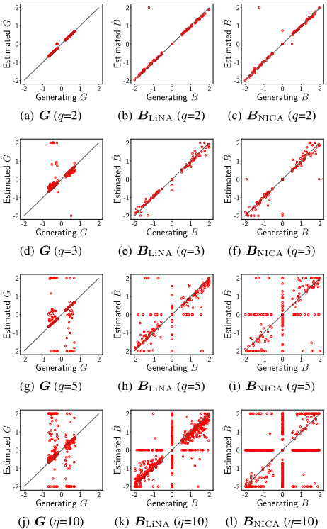
iii) Different numbers of latent factors q = 2, 3, 5, 10, to emphasize the capability of estimating causal effects, compared with NICA (Triad is not compared since it does not estimate effects). We applied the same method, CFA, to estimate ˆG as the NICA. Overall, in Figure 3, we found LiNA gives better performances in all cases. The accuracy decreases along with more latent factors. Specifically, NICA is comparable to ours when q = 2. However, as q = 10, accuracies both decrease, but LiNA decreases much more slowly than NICA. The reasons may be 1) more measurement variables with the fixed sample size results in reduced power of CFA to estimate ˆG, propagating errors to learn ˆB; 2) the sparsity constraint deals with small sample sizes while NICA does not. And NICA does not estimate the causal directions and effects simultaneously, which may lack statistical efficiency.

4 Average Variable Inflation Factors (VIF) are defined as the average VIF for all 100 independent trials of each range of weights.

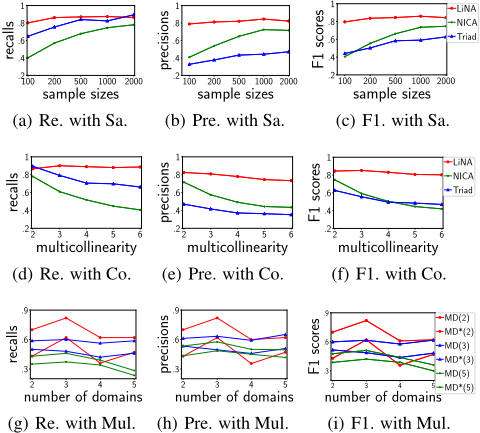
iv) Multi-domain data M = 2, 3, 4, 5, through varying noises ε's distributions (sub-Gaussian or super-Gaussian). To obtain the true graph for evaluation, we generated the identical graphs of latent factors in each domain. We varied the number of latent factors, qm = 2, 3, 5. In Figure 2(g)-(i), we found F1 scores of both methods tend to decrease with more domains or more latent factors increases. Specifically, in all cases MD-LiNA gives a better performance compared with MD*, in that MD* did neglect the problem that factors from different domains are represented by which factors of interest. Further, though we experimented with only qm = 2, 3, 5, the whole causal graph is much more complicated, which has totally Mqm latent factors and 2Mqm observed variables.

5.2 Real-World Applications

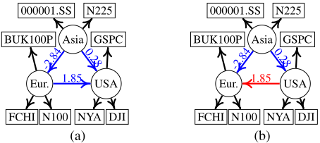
Yahoo stock indices dataset. We aimed to find the causal structure between different regions of the world, i.e., Asia, Europe, and the USA, each of which consisted of 2/3 stock indices. They were Asia := {N225, 000001.SS} from Japan and China, Europe := {BUK100P, FCHI,N100} from United Kingdom, France, and other European countries, and USA := {DJI,GSPC,NYA} from the United States. We divided the data into two non-overlapping time segments such that their distributions varied across segments and are viewed as two different domains. We tested its multicollinearity and used 10-fold cross validation to select parameter values. Details are in SM H.1. Due to the different time zones, it is expected the ground truth is Asia → Europe → USA [Janzing et al., 2010; Chen et al., 2014], with which our recovered causal structure in Figure 4 was in accordance.

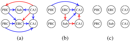
fMRI hippocampus dataset. We investigated causal relations between six brain regions of an individual: perirhinal cortex (PRC), parahippocampal cortex (PHC), entorhinal cortex (ERC), subiculum (Sub), CA1, and CA3/Dentate Gyrus (DG), each of which had left and right sides and were treated as measurements [Poldrack et al., 2015]. We used the anatomical connectivity between regions as a reference for evaluation [Bird and Burgess, 2008; Ghassami et al., 2018]. From Figure 5, we see though our method estimated one more redundant edge, we obtained more consistent as well as less spurious edges than NICA, while Triad failed to learn the relations between these regions in this data. Besides, we found our results also coincide with some current findings, e.g., ERC → CA1 is supposed to correlate with memory loss [Kerchner et al., 2012]. Please refer to SMH.2 for more details.

6 Conclusions

We proposed Multi-Domain Linear Non-Gaussian Acyclic Models for LAtent Factors (MD-LiNA) with its identification results, which gave deeper interpretation for latent factors that count. To discover the underlying causal structure for shared latent factors of interest, we proposed an integrated two-phase approach along with its local consistency. Our experimental results on simulated data and real-world applications validated the efficacy and robustness of the proposed algorithm.

Acknowledgments

This work was supported by the Grant ONR N00014-20-12501, the Natural Science Foundation of China (61876043, 61976052), Science and Technology Planning Project of Guangzhou (201902010058), and the Grant of China Scholarship Council. FX would like to acknowledge the support by China Postdoctoral Science Foundation (020M680225) and a research project of Huawei.