Reasoning-Based Learning of Interpretable ML Models

1 Introduction

The expanding reach of machine learning (ML) based systems and their complexity motivated the need for approaches that explain complex ML models. The quest for explainability of machine learning (ML) models has motivated in recent years a renewed interest in so-called interpretable ML models, namely in settings that are safety critical or where fairness and trust are required [Rudin, 2019]. Examples of ML models that are deemed interpretable include for instance decision trees [Nijssen and Fromont, 2007; Bessiere et al., 2009; Menickelly et al., 2016; Bertsimas and Dunn, 2017; Verwer and Zhang, 2017; Narodytska et al., 2018; Dash et al., 2018a; Verwer and Zhang, 2019; Aghaei et al., 2019; Hu et al., 2019; Lin et al., 2020; Avellaneda, 2020; Aglin et al., 2020a; Janota and Morgado, 2020; Zhu et al., 2020; Aglin et al., 2020b; Verhaeghe et al., 2020; Demirovic and Stuckey, 2020; Demirovic et al., 2020], lists [Angelino et al., 2017a; Angelino et al., 2017b; Rudin and Ertekin, 2018; Yu et al.,

2020a] and sets [F¨urnkranz et al., 2012; Lakkaraju et al., 2016; Ignatiev et al., 2018; Yu et al., 2020b; Ignatiev et al., 2021]. Nevertheless, there are other models that can also be viewed as interpretable, including (reduced) ordered binary decision diagrams [Bryant, 1986; Cabodi et al., 2021] ((R)OBDD), their well-known generalization of deterministic branching programs [Wegener, 2000], but also different knowledge representation languages [Audemard et al., 2020].

When learning interpretable models, one fundamental goal is to make the model as interpretable as possible. As a result, some measure of simplicity is often used, e.g. the size of the resulting model [Narodytska et al., 2018] or the sparseness of the model [Hu et al., 2019; Lin et al., 2020]. As a result, recent work focuses on learning models that offer some guarantee of optimality, e.g. size or accuracy.

For most interpretable models, concretely for those that are based on some sort of graph representation, the learning problem of an optimal model can be reduced to solving an NP decision problem. Indeed, given some goal in terms of representation size or accuracy, we just need to guess a representation respecting the size and the intended syntax (e.g. decision tree, list, set, etc.), and then check (in polynomial time on the size of the dataset and the representation) whether the representation matches the target goal. As a result, optimality can be achieved by iterative NP oracle calls, and so in practice, this problem has often been reduced to solving a sequence of instances of SAT. Moreover, the interest in the learning of interpretable ML models has led to dedicated approaches that bypass the encoding to a propositional representation [Hu et al., 2019; Aglin et al., 2020a; Lin et al., 2020; Aglin et al., 2020b; Verhaeghe et al., 2020; Demirovic and Stuckey, 2020; Demirovic et al., 2020].

This paper surveys the rapidly advancing area of learning optimal interpretable models, aiming at giving an accurate perspective of past work. The paper covers recent work on learning decision trees, sets and lists, but it also briefly overviews work on learning other models that can be deemed as interpretable [Audemard et al., 2020; Cabodi et al., 2021].

The paper is organized as follows. Section 2 introduces the definition and notation used in the rest of the paper, and overviews interpretable ML models. Section 3 overviews reasoning-based approaches. Afterwards, Section 4 discusses a number of additional trade-offs when learning optimal interpretable models. The paper concludes in Section 5.

2 Preliminaries &Models Overview

Classification problem. We start by defining the classification problem. An instance is a pair I = (fv, class), where fv ∈ Rn is a feature vector (f1, . . . , fn) and class is a class label, class ∈ K, where K is the set of possible class labels. Often we consider a binary classification problem, i.e. K = {⊖,⊕}. We denote the feature vector and class of an instance I as fv(I) and class(I), respectively. A dataset D is a set of instances: D = ∪k∈KDk , where the dataset Dk is the set of instances that belong to the kth class. In case of the binary classifier, we use datasets D⊕ and D⊖ to denote the sets of positive and negative instances. A classifier is a mapping f : fv → K. Given a dataset D and a classifier f, an instance I with class k = class(I) is misclassified if the classifier f incorrectly classifies instance I, i.e. f(fv(I)) = k′ , k′ ̸= k. Learning a classifier corresponds to selecting a function f from a family of functions aiming to maximise a given metric that we describe below. Next, we consider three classes of classifiers.

Decision tree (DT). Decision trees are binary trees, where each node is either a predicate node, which is assigned a predicate, or a classification node (leaf node), which is assigned to a class. A classification tree classifies an instance according to the following recursive procedure starting at the root node: if the node is a classification node, return the class assigned to the node, otherwise recurse on the left or right child node depending on the result of applying the instance to the node predicate. A common predicate choice is to evaluate whether a particular feature of the instances exceeds a threshold. The depth of a tree is the maximum number of predicates from the root node to any leaf node. The size of a tree is the number of nodes (predicate + classification) in the tree.

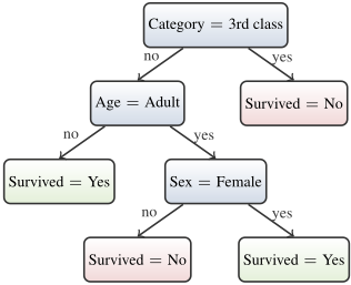
Example 1. Figure 1 shows an example of a DT for the Titanic dataset. Here, the DT is a binary classifier, i.e. all leaves are labeled with "No" or "Yes". A predicate node branches on whether a feature equals a certain value, e.g. whether the "Sex" feature of an individual is "Female" or "Male".

Decision set (DS). A decision set R is an unordered set of if-then rules of the from π ⇒ k, where π is a predicate and k is a class label, k ∈ K. Given an instance I and a rule π ⇒ k, if the instance satisfies the predicate π, i.e. π(I) = 1, then the rule predicts that I belong to class k. As rules in DSs are unordered, some rules may overlap, i.e. multiple rules' predicates may agree with an instance of the feature space. As such, one can either have a tie-break rule to pick the class [Lakkaraju et al., 2016] or declare an overlap [Ignatiev et al., 2018]. It may also happen that none of the rules of a DS apply to some instances. In this case, one can apply the default rule [Lakkaraju et al., 2016; Yu et al., 2020b].

Example 2. Figure 4a shows an example of a decision set for the Titanic dataset. Each rule consists of a predicate that constitutes a conjunction of constraints on features. For instance, the second rule is a conjunction of two unary constraints on features "Age" and "Sex". Namely, π := (Age = Adult) ∧ (Sex ̸= Female), The class label is "No" for this rule. If we have an instance (Age = Adult, Sex = Male, . . .) then the predicate π holds and we output class "No".

Decision list (DL). A decision list L = (r1, . . . , rP , r0) of length P ≥ 0 is a (P +1)-tuple consisting of P distinct rules πi ⇒ ki, i = 1, . . . , P, followed by a default rule r0. As above, a rule πi ⇒ ki corresponds to a conditional statement "if the predicate πi holds for a given instance then the class label is ki". The final default rule r0 of the DL can be seen as a special rule, where π0 = ⊤ so the predicate always holds.

Example 3. Figure 3a shows an example of a DL of length two for the Titanic dataset. Given an instance, the first rule's predicate checks whether features "Age" and "Sex" satisfy unary constraints. If so, the output label is "No". Otherwise, the second rule's predicate checks the "Category" feature of the instance. If Category ̸= 3rd class then we output "Yes". Otherwise, we apply the default rule and output "No".

Binarization. The language or predicates available to define decision trees, lists and sets is a crucial parameter of the methods. Most of the optimal methods we examine assume the features are binarized (one-hot encoding of categorical features, and binary representation of numerical features) and the predicates are simply the Boolean features themselves. We will point out where this assumption does not hold.

Optimization criteria. As mentioned above, learning a classifier is guided by an optimization function (or metric) specified by a user. For example, the user might prioritize the accuracy of the model over the its size or might want to consider a weighted combination of these criteria. Here we recall a few natural optimization metrics.

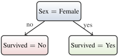
One metric to consider is the accuracy of the model. Accuracy is the ratio between the number of correctly classified instances and the number of all instances in the data. (Accuracy maximization can also be approached by minimizing the number of misclassifications.) The model is said to be perfect if it achieves highest possible accuracy on the training set. Note that the training data may contain conflicting instances I1 and I2, such that fv(I1) = fv(I2) and class(I1) ̸= class(I2). One option is to pre-process data and resolve conflicts using data statistics. Alternately, if we cannot resolve conflicts, we can keep these instances and let the classifier learn the best model. If the training data has no conflicting instances, a perfect model must classify all training data correctly, thus, yielding an accuracy of 100%; otherwise, the accuracy must be lower than 100%. Another important metric is model sparsity. For example, our optimization function can minimize the number of leaves in a tree or the depth of the tree. Figure 2 shows a sparse DT computed for the Titanic dataset. In case of DSs or DLs, we might want to optimize the number of rules or the number of constraints in predicates. Figures 4b and 3b show examples of a sparse DS and a sparse DL, respectively, for the same dataset. Note that the Titanic dataset has conflicting data instances with 78.25% of the data being non-conflicting. Thus, a perfect model achieves training accuracy of 78.25% on this dataset while sparse models' accuracy is guaranteed to be lower.

3 Reasoning-Based Approaches

3.1 Learning Decision Trees

Decision trees are one of the early influential approaches to ML. Original methods for creating decision trees were based on heuristics: CART [Breiman et al., 1984], ID3 [Quinlan, 1986] and C4.5 [Quinlan, 1993] - all build the tree iteratively by expanding a leaf node to improve some metric such as Gini impurity [Breiman, 1996] or information gain. Because these methods have a tendency to overfit, often some form of post-processing pruning is applied to reduce this [Bohanec and Bratko, 1994; Hastie et al., 2001].

The first approach we are aware of for building optimal misclassification decision trees, where the aim is to minimize the number of misclassified training instances is due to [Nijssen and Fromont, 2007]. Their DL8 algorithm is a dynamic programming approach to build optimal DTs, under various constraints, e.g. max depth. They restrict themselves, as does much of the work discussed in this section, to cases where features are all binary (by encoding if required). The dynamic programming nature of the problem arises because the optimal solution of the left subtree of a node and the right subtree are independent, once the split feature is determined. They make use of pattern mining methods to only examine branches that correspond to frequent itemsets.

[Bessiere et al., 2009] gave the first approach for DTs based on encoding to a discrete optimisation formalism, describing both a Boolean Satisfiability (SAT) and Constraint Programming (CP) model for building minimal size perfect decision trees which classify the training data perfectly. The CP model scaled much better then the SAT model although the authors apply subsampling of the data to increase scalability. They show the resulting decision trees are smaller than heuristic methods though not necessarily more accurate, and usually among the best methods in terms of accuracy.

[Bertsimas and Dunn, 2017] mapped the problem of building an optimal misclassification decision tree, restricted to complete trees of a given depth, to a Mixed Integer Program

(MIP). In this work the predicates fi ≥ d are used for splitting where d is part of the decisions. The resulting DTs were shown to be more (out-of-sample) accurate than those created by heuristic methods. The smaller the training set the better the accuracy over heuristic methods. The main limitation of the approach was scalability, it was able to handle problems with a few thousands training instances. While theoretically it could determine optimal DTs, in practice this only occurred for the smallest data sets or small depth limits.

Similar MIP approaches to the optimal classification DTs as well as optimal regression trees were developed by [Verwer and Zhang, 2017]. Improvements on these techniques were achieved [Verwer and Zhang, 2019] by essentially binarizing the training data, and restricting decisions to using these binary features. BinOct [Verwer and Zhang, 2019] was able to compute solutions much faster than the previous MIP methods, with increased accuracy (since it can more often find better solutions). A recent MIP approach [Zhu et al., 2020] improves on earlier MIP methods by using an SVM style objective to maximize the number of correctly classified instances, and introduces an LP based sample procedure to scale the approach to larger data sets, by selecting the most important instances to build the MIP model from. It selects the split predicates as part of the decisions.

A new SAT approach to computing smallest size perfect DTs was developed by [Narodytska et al., 2018], improving the encoding of [Bessiere et al., 2009] by simultaneously deciding the tree topology and feature decisions, and thus not only considering complete trees of some depth. The resulting SAT encodings were orders of magnitude smaller. The method is restricted by the number of training instances it can handle, and thus uses subsampling to handle large datasets. [Janota and Morgado, 2020] define an improved SAT model for perfect DTs, by explicitly encoding paths, rather than nodes in the tree. They add constraints to ensure the selected set of paths form a DT. Orthogonally [Avellaneda, 2020] gives a SAT approach that can minimize the size of the DT in terms of nodes, and shows how to use active learning to improve the training time. [Hu et al., 2020] extend the SAT model of [Narodytska et al., 2018] in a MaxSAT solution to directly optimise for size of a perfect DT. They also show how to use MaxSAT to reduce overfitting by optimal boosting.

[Verhaeghe et al., 2020] developed a CP approach to constructing an optimal misclassification DT of bounded depth, by combining global constraints developed for itemset mining with a form of AND/OR tree search and caching to define a flexible approach to DT construction similar in broad details to a dynamic programming approach. They show that the CP approach is superior in construction time to previous methods DL8 and BinOCT that can answer the same question.

This CP approach was improved in the DL8.5 system [Aglin et al., 2020a] by replacing the CP solver with a bespoke branch and bound caching AND/OR tree search, essentially a dynamic programming solution. The approach combines pruning based on depth, minimum support, purity (all remaining examples are in one class) and pruning the right child using the answers from the left. It outperformed previous methods by an order of magnitude, and was further improved by using sparse bit vectors [Aglin et al., 2020b].

Further improvements to the branch and bound dynamic programming approach were given in [Demirovic and Stuckey, 2020]. They noticed that the optimal depth 2 trees can be computed in O(m2 |D|) rather than O(n2 |D|) where m is the maximal number of positive features appearing in any instance, thus improving the base case for the dynamic program. This together with extensions to directly bound the size (rather than only depth) and use nearby cached solutions to compute lower bounds improved runtime compared to DL8.5 [Aglin et al., 2020b] by orders of magnitude.

In a slightly different direction [Hu et al., 2019] presented a branch and bound dynamic programming approach for computing optimal sparse DTs, where each node in the tree is considered as equal to some number of misclassifications. This approach avoids the need for a depth bound assumed in other methods, bounding the size of the tree using the sparsity objective. The resulting trees report very high accuracy, since sparsity acts as a strong regularizer.

Overall building optimal DTs using bespoke branch and bound approaches is reasonably scalable, since the methods are linear in the training data. The bottlenecks arise from the number of features and the maximum size or depth of the tree.

3.2 Learning Decision Lists

Decision lists were introduced by Rivest (1987) and heuristic methods for decision lists also date back to the late 80s, e.g. CN2 [Clark and Niblett, 1989; Clark and Boswell, 1991].

One recent approach [Angelino et al., 2017a; Rudin and Ertekin, 2018] provides DLs that have some optimality guarantee. Given a fixed set of decision rules, it chooses a minimum-size ordered subset of these rules; the order essentially terminates when a default rule is chosen. The authors model the problems as an integer program (IP) and solve it with a mixed integer programming (MIP) solver. The objective is a combination of training accuracy and sparsity, minimizing misclassifications where every used rule incurs a "cost" of C misclassifications, and every used literal costs C1 misclassifications. The method exhibits scalability issues and it is somewhat restricted by the time required to generate all potential possible rules as input. They consider data sets with up to 3000 examples and 60 features, but cannot prove optimality of their solutions on the data tested. One advantage of the approach is that it is easy to customize, e.g. favoring the use of certain features, or extending to cost-sensitive learning.

To the best of our knowledge, the first method to generate optimal decision lists extends the approach of [Rudin and Ertekin, 2018] using the same idea of ordering a fixed set of decision rules, but using a bespoke branch-and-bound algorithm [Angelino et al., 2017b]. The method makes use of bounding methods and symmetry elimination techniques. They minimize regularized misclassification, where each rule costs λM misclassification errors where M is the number of training examples. The approach relies on the sparsification parameter λ to limit the set of rules it needs to consider. It can find and prove optimal solutions to large problems (hundreds of thousands of examples), the main limitation is on the number of features, since the number of possible decision rules grows exponentially in the number of features.

A novel SAT- and MaxSAT-based approach to learning perfect and sparse DLs was proposed in [Yu et al., 2020a]. It builds on the prior work on training perfect and sparse DSs [Ignatiev et al., 2018; Yu et al., 2020b], targets minimization of the total number of literals in use and is shown to scale similarly to [Yu et al., 2020b]. The approach is compared against optimal perfect and sparse DSs as well as the earlier DL inference approach CORELS of [Angelino et al., 2017a; Angelino et al., 2017b]. It is able to produce DLs that are guaranteed to be optimal with respect to the metric in use. Note that sparse DLs are computed using the constant regularization parameter λ that indicates how much misclassifications a given literal costs if added to the DL model.

3.3 Learning Decision Sets

Decision sets are a rule-based predictive model that can be traced at least to the work on heuristic algorithms CN2 [Clark and Niblett, 1989; Clark and Boswell, 1991] and RIPPER [Cohen, 1995]. To the best of our knowledge, decision sets first appear as an unordered variant of DLs [Rivest, 1987; Clark and Niblett, 1989] in [Clark and Boswell, 1991].

The use of logic and optimization for synthesizing a disjunction of rules matching a given training dataset was first proposed in [Kamath et al., 1992]. This work targets solely binary classification problems and focuses on computing an explicit formula representing one class (either ⊕ or ⊖). Each rule is assumed to be a conjunction of feature literals, i.e. the classifier is computed in the form of disjunctive normal form (DNF) (similar reasoning can be applied for inferring CNF representations). Concretely, they propose a CNF encoding for computing such a target formula representation, which is then tackled with the use of the interior point method.

Recently, [Ignatiev et al., 2018] proposed a few problem formulations for computing smallest size perfect DSs with an explicit representation of each of the multiple classes. They vary in terms of how rule overlap is handled, which leads to the varying problem complexity for the proposed variants. The work also proposes a novel SAT encoding for minimizing the number of rules in the target DS using a sequence of SAT oracle calls. Each such oracle call decides whether or not a DS of a given size exists. The approach of [Ignatiev et al., 2018] is shown to significantly outperform the smooth local search approach, proposed earlier in [Lakkaraju et al., 2016].

Although the number of rules is a valid metric for measuring DS size, in practice a user may get a DS with a small number of rules such that each rule has a large size. This makes it hard for a user to interpret the predictions made by the model. As a result, [Ignatiev et al., 2018] extends the SAT-based approach to rule minimization with an additional step to minimize the total number of literals used in the DS, which results in a lexicographic approach to minimization.

In contrast, [Yu et al., 2020b] builds on the approach of [Ignatiev et al., 2018] but instead for the first time proposes to directly minimize the total number of literals in the target DS. Unsurprisingly, they confirm that minimizing the number of rules is more scalable for solving the perfect DS problem since the optimization measure, i.e. the number of rules, is more coarse-grained. However, minimizing the total number of literals is shown to produce significantly smaller and, thus, more interpretable DSs. They also extend the approach to

(a) An example smallest size perfect decision list learned by [Yu et al., 2020a], with training accuracy 78.25%.

(b) An example sparse decision list learned by [Angelino et al., 2017a], with training accuracy 70.69%.

• (a) An example smallest size perfect decision set learned by [Ignatiev et al., 2021], with training accuracy 78.25%.

(b) An example sparse decision set learned by [Yu et al., 2020b], with training accuracy 77.57%.

Figure 4: Example decision sets for the well-known Titanic dataset. Both decision sets are computed by minimizing the number of literals.

sparse DSs (minimizing either of the metrics) provide a user with yet another way to produce a succinct classifier representation, by trading off its accuracy for smaller size (an example sparse DS computed by the method of [Yu et al., 2020b] for the Titanic dataset is shown in Figure 4b).

Sparse DSs are also considered in [Malioutov and Meel, 2018; Ghosh and Meel, 2019] where the authors propose a MaxSAT model for representing one target class of the training data, and the size of the model is measured as the total number of literals across all rules. As such, rather than building a perfect DS classifier, they consider a model representing a single class that minimizes a linear combination of size and Hamming loss, to control the trade-off between accuracy and size. Note that this approach assumes the number of rules to be constant and to be provided by a user, i.e. they do not guarantee to produce an optimal DS with respect to the total size of the DS. Scalability of this approach is improved in [Ghosh and Meel, 2019], which proposes to learn rules iteratively on partitions of the training set. Note that they do not create a decision set as defined in [Clark and Boswell, 1991; Lakkaraju et al., 2016; Ignatiev et al., 2018], but rather a single formula that defines one of the classes, e.g. ⊕. (Observe that the ⊖ instances are specified by default as the instances not captured by the ⊕ formula.) This limits the approach of [Malioutov and Meel, 2018; Ghosh and Meel, 2019] to binary classification, and also makes the representation smaller. The lack of explicit representation for one of the two target classes also means that explainability is reduced for the data instances of the "unrepresented" class, since a user has to use the (negation of the) entire formula for the "represented" class to explain the classification. This line of work is further extended in [Ghosh et al., 2020] where the concept of a rule in relaxed form is introduced based on relaxed definitions of the standard {∧, ∨} operations. This work argues that the classifiers based on the relaxed rules are more succinct and accurate than the standard DNF- and CNF-based models.

Integer Programming (IP) has also been used to create optimal DS models that only have positive rules. [Dash et al., 2018b] proposes an IP model for binary classification, where an example is classified as ⊕ if and only if it satisfies at least one clause of the model. The IP model minimizes a variation on the Hamming loss, which is the number of incorrectly classified ⊕ examples, plus, for each incorrectly classified ⊖ example, the number of clauses incorrectly classifying it. The complexity of the model is controlled by a bound on the size of each clause. The IP model has one binary variable for each possible clause and the authors use column generation [Barnhart et al., 1998]. Even so, as the pricing problem can be too expensive, it is solved heuristically for large datasets.

The perfect DSs of [Ignatiev et al., 2018] and sparse DSs of [Malioutov and Meel, 2018; Ghosh and Meel, 2019] are compared in [Yu et al., 2020b] in terms of runtime performance but also in terms of model and explanation size. One of their main conclusions is that perfect DSs are (in some cases significantly) larger than sparse DSs, which in turn deteriorates the performance of the perfect models due to encoding size. Model size also affects interpretability of perfect DSs as the smaller the model is the easier it is to comprehend for a human decision maker. ([Yu et al., 2020b] also argues that best model size and so best model interpretability is achieved by the models targeting minimization of the total number of literals [Yu et al., 2020b] rather than minimization of the number of rules [Ignatiev et al., 2018]; in this sense, the lexicographic approach of [Ignatiev et al., 2018] is also shown to perform reasonably well.) On the other hand, perfect DSs of [Ignatiev et al., 2018; Yu et al., 2020b] outperform their sparse counterparts wrt. training accuracy, which is not surprising given that perfect models aim at complying with the largest portion of the training data. (This conclusion on the better accuracy achieved by perfect models is later extended to the test accuracy in [Yu et al., 2020a].)

Finally, one of the latests reasoning-based approaches to training perfect DSs is proposed in [Ignatiev et al., 2021], where the training process is split into two separate phases: (1) enumerating individual rules exhaustively with the use of incremental MaxSAT followed by (2) solving the set cover problem with a MIP solver, to select an optimal subset of collected rules that match the training data. The approach is also strengthened by applying effective symmetry breaking used to reduce the number of rules enumerated in phase 1. An advantage of this approach is that a user can apply it to minimize either the number of rules or the number of literals, simply by selecting the objective function in phase 2 of the approach. Also, the two-phase approach is shown to outperform all the state-of-the-art competitors in perfect DS learning by a few orders of magnitude, including prior works [Ignatiev et al., 2018; Yu et al., 2020b]. However, this approach suffers from the lack of support for sparse DSs - adapting it to the sparse setting may result in a highly efficient method of training sparse DSs but it is yet to be investigated.

4 Additional Remarks

This section summarizes the discussion of the previous sections and makes a few more observations regarding the reasoning-based approaches to interpretable ML models.

Comparing toHeuristicMethods. Themethods discussed here demonstrate that the resulting models (including DTs, DLs, and DSs) typically have much higher out-of-sample accuracy than heuristic approaches, even than more expressive methods such as random forests. The training times are typically higher than heuristic approaches, but over the evolution of the methods the difference has drastically narrowed.

Other Interpretable Models. [Cabodi et al., 2021] investigated two approaches for learning OBDDs [Bryant, 1986]. One approach is based on encoding the learning problem into SAT. (This is outlined in Section 1 for most ML models that are based on a directed acyclic graph representation, e.g. deterministic branching programs [Wegener, 2000] or any of their restrictions, including decision trees, BDDs, etc.) Another approach taps on the large body of work on reasoning about BDDs [Bryant, 1986; Wegener, 2000], and proposes a heuristic approach for learning an OBDD from a dataset.

Perfect vs Sparse Models. Many approaches have been proposed in the recent past to all the major rule-based models, including DTs, DLs, and DSs. More importantly, for all them there are methods that aim at perfectly accurate classification but also approaches that focus on various sparsity criteria instead. In general, sparse models are deemed to be easier to compute due to their smaller size (and thus smaller formal encoding). They are shown to generalize well on unseen data and provide a user with a reasonably good test accuracy. Additionally, smaller model size overall implies that explanation size on average is smaller for sparse models. On the other hand, perfect models provide the highest possible training accuracy, which may in some settings be crucial.

Model Expressivity and Size. When learning interpretable models, some initial results are known [Rivest, 1987]. Concretely, DLs are more succint than DTs, and DLs are more succint than DNFs, i.e. a very special case of a DS. To the best of our knowledge, there are also a number of open problems. It is unclear how to categorize DSs. The relation between DTs and OBDDs is also unclear [Zantema and Bodlaender, 2002]. No results are known comparing DLs with OBDDs.

Although we are unaware of any practical works comparing DTs against DLs or DSs, [Yu et al., 2020a] reports initial empirical results confirming that DLs are in general more succinct than DSs if trained on the same datasets. Note that this was reported to hold both for perfect and sparse models.

Interpretability. Despite the lack of work comparing DTs, DLs, and DSs from the perspective of model interpretability, [Yu et al., 2020a] provides initial considerations on comparative interpretability of DLs and DSs. The authors propose a few metrics for measuring an explanation for DL and DS models. Their findings suggest although perfect DLs are typically more succinct than perfect DSs, the explanations for perfect DLs are on average longer than those for perfect DSs. On the contrary, sparse DLs are shown to outdo sparse DSs in terms of average explanation size. Also, [Yu et al., 2020a] compares with the explanation size for optimal sparse DLs of [Angelino et al., 2017a; Rudin and Ertekin, 2018] and indicate the that optimality measure exploited by [Yu et al., 2020a] enables one to train more interpretable models.

[Izza et al., 2020] is devoted to computing minimal conjunctive (PI-)explanations [Shih et al., 2018; Ignatiev et al., 2019] to DT predictions. Conventionally, an explanation for a prediction in a DT can be associated with a path executed in the tree for a data instance to be classified. The authors argue that although decision trees are deemed to be one of the most interpretable models, in practice PI-explanations may be arbitrarily smaller than "default" explanations computed as paths firing the prediction, even if the target DTs are guaranteed to be of minimum size. It is yet unclear whether or not similar observations can be made for DLs and DSs.

Fairness and Other Constraints. One of the principle advantages of using reasoning for building ML models is that additional constraints may be added to enforce some property of the resulting ML model. [Aghaei et al., 2019] defined a MIP formulation for optimal DTs that included fairness metrics, thus guaranteeing the resulting decision tree met some measure of fairness. They do require high computation time compared to specialised heuristic methods for the same problem, e.g. [Kamiran et al., 2010]. Other interpretable models have also been used in the context of fairness. For example, [Ignatiev et al., 2020] showed how to learn fair decision sets, starting fromeither biased or unbiased datasets. In both cases, the key insight is that one can trade off accuracy for fairness.

5 Conclusions

With the growing awareness of the importance of explainability of ML models, there has been renewed interest in learning interpretable models, including decision trees, lists and sets, among others. Moreover, such interest focused on learning optimal ML models, using different definitions of optimality, which offer stronger guarantees in terms of interpretability. This paper surveys the main results in reasoning-based learning optimal interpretable models, covering work since the late 80s, but also highlighting the most recent advances. Given the importance of the topic, one should expect additional improvements and results in the near future.

Acknowledgements

This work is supported by the AI Interdisciplinary Institute ANITI, funded by the French program "Investing for the Future - PIA3" under Grant agreement no ANR-19-PI3A-0004.