
A Universal PINNs Method for Solving Partial Differential Equations with a Point Source
Proceedings of the Thirty-First International Joint Conference on Artificial Intelligence. Main Track. Pages 3839-3846.
https://doi.org/10.24963/ijcai.2022/533
Keywords
- Multidisciplinary Topics and Applications: Physical Science
- Machine Learning: Multi-task and Transfer Learning
- Machine Learning: Unsupervised Learning
Abstract
In recent years, deep learning technology has been used to solve partial differential equations (PDEs), among which the physics-informed neural networks (PINNs)method emerges to be a promising method for solving both forward and inverse PDE problems. PDEs with a point source that is expressed as a Dirac delta function in the governing equations are mathematical models of many physical processes. However, they cannot be solved directly by conventional PINNs method due to the singularity brought by the Dirac delta function. In this paper, we propose a universal solution to tackle this problem by proposing three novel techniques. Firstly the Dirac delta function is modeled as a continuous probability density function to eliminate the singularity at the point source; secondly a lower bound constrained uncertainty weighting algorithm is proposed to balance the physics-informed loss terms of point source area and the remaining areas; and thirdly a multi-scale deep neural network with periodic activation function is used to improve the accuracy and convergence speed. We evaluate the proposed method with three representative PDEs, and the experimental results show that our method outperforms existing deep learning based methods with respect to the accuracy, the efficiency and the versatility.
- [Bekele, 2020] Yared W Bekele. Physics-informed deep learning for flow and deformation in poroelastic media. arXiv preprint arXiv:2010.15426, 2020.
- [Bischof and Kraus, 2021] Rafael Bischof and Michael Kraus. Multi-objective loss balancing for physics- informed deep learning. arXiv preprint arXiv:2110.09813, 2021.
- [Cai et al., 2021] Shengze Cai, Zhicheng Wang, Sifan Wang, Paris Perdikaris, and George Em Karniadakis. Physics- informed neural networks for heat transfer problems. Jour- nal of Heat Transfer, 143(6):060801, 2021.
- [Gedney, 2011] Stephen D Gedney. Introduction to the finite-difference time-domain (fdtd) method for electro- magnetics. Synthesis Lectures on Computational Electro- magnetics, 6(1):1-250, 2011.
- [He et al., 2016] Kaiming He, Xiangyu Zhang, Shaoqing Ren, and Jian Sun. Deep residual learning for image recog- nition. In Proceedings of the IEEE conference on computer vision and pattern recognition, pages 770-778, 2016.
- [Hennigh et al., 2021] Oliver Hennigh, Susheela Narasimhan, Mohammad Amin Nabian, Akshay Subra- maniam, Kaustubh Tangsali, Zhiwei Fang, Max Rietmann, Wonmin Byeon, and Sanjay Choudhry. Nvidia simnet™: An ai-accelerated multi-physics simulation framework. In International Conference on Computational Science, pages 447-461. Springer, 2021.
- [Heydari et al., 2019] A Ali Heydari, Craig A Thompson, and Asif Mehmood. Softadapt: Techniques for adap- tive loss weighting of neural networks with multi-part loss functions. arXiv preprint arXiv:1912.12355, 2019.
- [Jin et al., 2021] Xiaowei Jin, Shengze Cai, Hui Li, and George Em Karniadakis. Nsfnets (navier-stokes flow nets): Physics-informed neural networks for the incom- pressible navier-stokes equations. Journal of Computa- tional Physics, 426:109951, 2021.
- [Kendall et al., 2018] Alex Kendall, Yarin Gal, and Roberto Cipolla. Multi-task learning using uncertainty to weigh losses for scene geometry and semantics. In Proceedings of the IEEE conference on computer vision and pattern recognition, pages 7482-7491, 2018.
- [Li et al., 2020] Zongyi Li, Nikola Kovachki, Kamyar Az- izzadenesheli, Burigede Liu, Kaushik Bhattacharya, An- drew Stuart, and Anima Anandkumar. Fourier neural op- erator for parametric partial differential equations. arXiv preprint arXiv:2010.08895, 2020.
- [Liu et al., 2020] Ziqi Liu, Wei Cai, and Zhi-Qin John Xu. Multi-scale deep neural network (mscalednn) for solving poisson-boltzmann equation in complex domains. arXiv preprint arXiv:2007.11207, 2020.
- [Lu et al., 2019] Lu Lu, Pengzhan Jin, and George Em Kar- niadakis. Deeponet: Learning nonlinear operators for identifying differential equations based on the univer- sal approximation theorem of operators. arXiv preprint arXiv:1910.03193, 2019.
- [McClenny and Braga-Neto, 2020] Levi McClenny and Ulisses Braga-Neto. Self-adaptive physics-informed neural networks using a soft attention mechanism. arXiv preprint arXiv:2009.04544, 2020.
- [Moseley et al., 2020] Ben Moseley, Andrew Markham, and Tarje Nissen-Meyer. Solving the wave equation with physics-informed deep learning. arXiv preprint arXiv:2006.11894, 2020.
- [Pinkus, 1999] Allan Pinkus. Approximation theory of the mlp model. Acta Numerica 1999: Volume 8, 8:143-195, 1999.
- [Raissi et al., 2019] Maziar Raissi, Paris Perdikaris, and George E Karniadakis. Physics-informed neural networks: A deep learning framework for solving forward and in- verse problems involving nonlinear partial differential equations. Journal of Computational Physics, 378:686- 707, 2019.
- [Sirignano and Spiliopoulos, 2018] Justin Sirignano and Konstantinos Spiliopoulos. Dgm: A deep learning algo- rithm for solving partial differential equations. Journal of computational physics, 375:1339-1364, 2018.
- [Sitzmann et al., 2020] Vincent Sitzmann, Julien Martel, Alexander Bergman, David Lindell, and Gordon Wet- zstein. Implicit neural representations with periodic ac- tivation functions. Advances in Neural Information Pro- cessing Systems, 33, 2020.
- [Sullivan, 2013] Dennis M Sullivan. Electromagnetic simu- lation using the FDTD method. John Wiley & Sons, 2013.
- [Wang et al., 2020] Sifan Wang, Xinling Yu, and Paris Perdikaris. When and why pinns fail to train: A neural tan- gent kernel perspective. arXiv preprint arXiv:2007.14527, 2020.
- [Wang et al., 2021] Sifan Wang, Yujun Teng, and Paris Perdikaris. Understanding and mitigating gradient flow pathologies in physics-informed neural networks. SIAM Journal on Scientific Computing, 43(5):A3055-A3081, 2021.
- [Weinan and Yu, 2018] E Weinan and Bing Yu. The deep ritz method: a deep learning-based numerical algorithm for solving variational problems. Communications in Math- ematics and Statistics, 6(1):1-12, 2018.
- [Xu et al., 2019] Zhi-Qin John Xu, Yaoyu Zhang, Tao Luo, Yanyang Xiao, and Zheng Ma. Frequency principle: Fourier analysis sheds light on deep neural networks. arXiv preprint arXiv:1901.06523, 2019.
- [Zhang et al., 2021] Pan Zhang, Yanyan Hu, Yuchen Jin, Shaogui Deng, Xuqing Wu, and Jiefu Chen. A maxwell's equations based deep learning method for time domain electromagnetic simulations. IEEE Journal on Multi- scale and Multiphysics Computational Techniques, 6:35- 40, 2021.
References were extracted automatically from the PDF and may contain errors.
Full text extracted automatically from the PDF; figures, tables and equations may differ. The PDF is the version of record.
1 Introduction
Partial differential equations (PDEs) play a significant role in science and engineering disciplines, which are used to formulate physical problems such as sound propagation, fluid flow, electromagnetic field, etc. In the past decades, numerical methods of PDEs have been developed and successfully applied to many real-world applications like aerodynamics and weather forecasting. However, as the scale and complexity of the problem increase, the computational complexity of numerical methods becomes prohibitively high.
∗Corresponding author
On the other hand, with the increase use of numerical methods in both industry and academia, a growth in the collection of simulation data has been observed in computational fluid dynamics, electromagnetic simulation and many other areas, and data-driven deep learning approaches [Lu et al., 2019; Li et al., 2020] are proposed to alleviate the computational burden. Data-driven deep learning methods have the advantage that once the neural network is trained, the prediction process is fast. However, the cost of data acquisition is prohibitive for complex physical, biological, and engineering systems, and the generalization ability of the model (from one experimental condition to another) is poor when there are not sufficient labeled data [Cai et al., 2021]. Therefore, physics-informed methods have been proposed in recent years that rely on the universal approximation ability of deep neural network [Pinkus, 1999] and automatic differentiation of the deep learning frameworks. Compared with traditional PDE solvers, deep learning solvers [Sirignano and Spiliopoulos, 2018; Weinan and Yu, 2018; Raissi et al., 2019] can not only deal with parametrized simulations, but also address the inverse or data assimilation problems that traditional solvers cannot deal with. Among these methods, the physics-informed neural networks (PINNs) method [Raissi et al., 2019] attracts increasing attentions from machine learning and applied mathematics communities due to its simple and effective way of approximating the solutions of PDEs using neural networks. The PINNs method preserves physical information in the governing equations and adapts to the boundary conditions. The PINNs method has been applied to solve many well-known PDEs such as Navier-Stokes equations [Jin et al., 2021] and Maxwell's equations [Zhang et al., 2021].
PDEs with a point source expressed as a Dirac delta function δ(x) have many applications in physical simulation. For instance, a point source can be a pulse exciting the electric field in electromagnetic simulation [Sullivan, 2013], or a sound source in an acoustic wave equation [Moseley et al., 2020]. However, conventional PINNs method reviewed above cannot be directly used to solve this problem due to the singularity brought by the Dirac delta function. Several methods have been proposed in the literature to solve this problem under certain constraints. For example, the Deep Ritz method [Weinan and Yu, 2018] and the variational method in NVIDIA SimNet [Hennigh et al., 2021] need to transform the point source term into a computer computable form, which however is not applicable to all PDEs with a point source; PINNs-based methods proposed by [Zhang et al., 2021; Moseley et al., 2020; Bekele, 2020] require some labeled data as an additional loss term that may not be available in some cases.
In this paper, we propose a universal approach to solve PDEs with a point source based on the PINNs method. Our approach does not rely on any labeled data or variational forms, and meanwhile outperforms existing deep learning based methods with respect to the accuracy, the efficiency and the versatility. Our method employs three novel techniques:
- A continuous unimodal probability density function is used to model the Dirac delta function to eliminate the singularity at the point source;
- A lower bound constrained uncertainty weighting algorithm is proposed to balance the loss terms of the point source area and the remaining areas;
- A neural network architecture is built with multi-scale DNN [Xu et al., 2019] and periodic activation functions to improve the accuracy and convergence speed of the PINNs method.
2 Preliminaries
The general form of a time-dependent PDE is given by:
where N(·) is the differential operator, u is the solution, and f(x, t) is the time-dependent forcing term. For PDEs with a point source that we consider in this paper, the forcing term f(x, t) contains the Dirac delta functions.
2.1 PDEs with a Point Source
Here we introduce two well-known time-(in)dependent PDEs with a point source forcing term. The Poisson's equation with a point source has the following form:
where δ denotes the Dirac delta function. In the field of electromagnetic simulations, the time domain Maxwell's equations with excitation can be expressed as
where ϵ is the permittivity, µ is the permeability. The forcing term J(x, t) = δ(x - x0)g(t) excites a wave propagation at x0 with a particular type of pulse g(t).
2.2 The PINNs Method
In order to solve PDE problems with deep learning technology, the PINNs method is proposed to approximate the solution u(x, t) with a deep neural network u(x, t; θ), where θ represents the trainable parameters of the deep neural network. The loss function given by such approximation is defined as
where Lr, Lic, Lbc correspond to the loss term of PDE residual, initial conditions, and boundary conditions, respectively. The hyperparameters λic and λbc aim to balance the interplay of different terms in the loss function. Nr, Nic, and Nbc represent the number of samples in the entire region, initial conditions, and boundary conditions, respectively.
When f(·), g(·), h(·) are continuous, the network weights θ can be optimized by minimizing the total training loss Ltotal(θ) via standard gradient descent procedures used in deep learning. Unfortunately, due to the singularity brought by δ(x), the PINNs method cannot be directly used to solve the PDEs with a point source.
2.3 RelatedWorks
One can use the Deep Ritz method [Weinan and Yu, 2018] to solve Eq.(2). Through mathematical derivation, Eq.(2) can be converted to the following minimization problem:
where the Dirac function term δ(x-x0) in Eq.(2) will generate the constant term u(x0) in Eq.(5) after integration. However, the Deep Ritz method is unable to solve PDEs like Eq.(3) that cannot be derived from any variational problem. The NVIDIA SimNet [Hennigh et al., 2021] uses variational formulation to solve PDEs with a point source. However, its performance heavily depends on the selection of the test functions and the computational time increases linearly with the number of test functions.
[Zhang et al., 2021] and [Moseley et al., 2020] use classical numerical method to simulate the early period (0 ≤ t ≤ T0 < T) of wave equations to avoid point source singularity, and then applied the PINNs method to solve the PDEs with given initial conditions at t = T0. [Bekele, 2020] attempted to leverage the PINNs loss by adding a new loss term with a significant amount of known labels when solving the Barry and Mercer's source problem with time-dependent fluid injection. However, these methods rely on classical computational methods to generate the labeled data which is expensive or even infeasible in many situations.
In this work, we propose a universal solution based on the PINNs method that does not rely on any labeled data or variational forms.
3 Methodology
In this section, we explain our strategy to tackle the singularity problem in detail.
3.1 Approximation to δ(x)
The Dirac delta function δ(x) is mathematically defined by:
Taking η(x) to be any symmetric unimodal continuous probability density function centered at 0, η(x) = α-1 η( xα ) can be a natural approximation to δ(x) as the kernel width α → 0. In a d-dimensions space, ηα(x) = α-d η( xα ) can be used instead. In our experiments, we use Gaussian distribution, Cauchy distribution and Laplacian distribution with sufficiently small kernel width α to approximate δ(x).
3.2 Lower Bound Constrained Uncertainty Weighting
Our approximation to δ(x) eliminates function discontinuity at the origin, but it also brings a difficulty for the PINNs method to optimize its training loss. As the probability density function is highly concentrated at the origin as α → 0, the residual samples close to the origin tend to dominate the whole residual loss, making it difficult for the network to learn the governing equations and therefore the standard optimizer may not converge to the solution. To address this problem, we split the feasible region into two subdomains such that:
where Ω0 represents the subdomain that contains the origin and Ω1 covers the complement region. By taking this decomposition, the residual loss Lr in Eq.(4) is divided into two parts:
where Lr,0(θ) and Lr,1(θ) correspond to the residual losses in Ω0 and Ω1, respectively. In our experiment, for the point source excited at x0 ∈ Ω, we split Ω as
Together with the IC&BC conditions, the total PINNs loss in Eq.(4a) changes to be:
Properly setting the weight vector λ = (λr,0, λr,1, λic, λbc) is critical to enhance the trainability of constrained neural networks [McClenny and Braga-Neto, 2020; Wang et al., 2020], but searching the optimal weight vector through manual tuning is infeasible.
In multi-task learning, different tasks share the same backbone network but correspond to different loss terms. These loss terms need to be weighted to balance their contributions to the total loss during training. Several algorithms [Kendall et al., 2018; Heydari et al., 2019] have been proposed to solve the loss weighting problem in multi-task learning, and some of them are utilized in PINNs method. Specifically, [Wang et al., 2021] propose a learning rate annealing algorithm that uses back-propagation gradient statistics in the training process to adaptively balance the contribution of each loss term, and [Bischof and Kraus, 2021] propose ReLoBRaLo method to perform loss weighting based on the SoftAdapt method proposed by [Heydari et al., 2019].
In this work, we adapt the uncertainty weighing method in [Kendall et al., 2018] to solve the problem. Specifically, for a total loss function including m loss terms L(θ) = ∑mi=1 λiLi(θ), we add a nonnegative ϵ2 to w2 , and get the total PINNs loss function as follows:
The uncertainty of the i-th loss term is approximated by ϵ2 + w2 i , whose lower bound is constrainted by ϵ2 when decreasing wi to 0. We argue that such reformulation is nontrivial since it provides a lower bound for the uncertainty estimation of each loss term and thus increases the stability of the self-adaptive weighting algorithm.
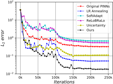
Fig.1 shows the convergence process of the mean L2 errors with different loss weighting methods in solving Barry and Mercer's source problem. It shows that our lower bound constrained uncertainty weighting method outperforms other methods. SoftAdapt [Heydari et al., 2019] and ReLoBRaLo [Bischof and Kraus, 2021] methods both fail to converge to good accuracies in this scenario, even worse than the equally weighted PINNs method ('Original PINNs'). We believe this is due to the extreme imbalance between Lr,0(θ) and other loss terms, whereas SoftAdapt and ReLoBRaLo can only deal with cases where differences between loss terms are not significant. The learning rate annealing algorithm ('LR Annealing') is better than the original uncertainty weighting method ('Uncertainty') [Kendall et al., 2018], but worse than our proposed method. It is worth noting that the learning rate annealing algorithm requires the back-propagation gradient statistics, which brings additional training time overhead.
3.3 Multi-Scale DNNs with Periodic Activation Function
For a 2-D Possion's equation with a point source located at (x0, y0) within a domain Ω = (0, π)2 , the analytical solution is as follows:
The analytical solution is formed by superposition of multiple frequency components. This multi-frequency phenomenon is common in solutions of many PDEs. Recent development in deep learning theories [Xu et al., 2019] reveals that the neural network fits the hidden physical law from low to high frequency components. Based on this theory, [Liu et al., 2020] proposes multi-scale deep neural networks (MscaleDNNs) which exhibit faster convergence in higher frequency components.
Periodic nonlinearity has been extensively investigated over the past decades. Recently SIREN architecture [Sitzmann et al., 2020] is proposed to use Sine function as a periodic activation function and outperforms alternative activation functions when dealing with implicit neural representations and their derivatives. Compared with other activation functions, e.g., Tanh and ReLU, derivative of a Sine function is Cosine, a phase-shifted Sine. Therefore, derivatives of a SIREN inherit the SIREN's properties, thus enabling us to supervise any derivative of SIREN with complex natural signals from PDEs.
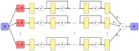
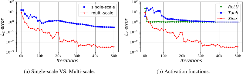
Borrowing ideas from MscaleDNNs and SIREN, we propose Multi-Scale SIREN (MS-SIREN) that combines multiscale DNNs with Sine activation function, as shown in Fig.2. Skip connections are added between consecutive hidden layers to accelerate training and improve accuracy as they help to avoid the vanishing gradient problem [He et al., 2016]. Fig.3 shows the effectiveness of MS-SIREN compared with other alternative architectures.
| Network Architectures | L2 error | |||||
|---|---|---|---|---|---|---|
| # subnets | # layers | # neurons | Ex | Ey | Hz | mean |
| 1 | 7 | 256 | 0.192 | 0.183 | 0.433 | 0.269 |
| 1 | 9 | 256 | 0.147 | 0.146 | 0.070 | 0.121 |
| 2 | 7 | 128 | 0.079 | 0.074 | 0.058 | 0.072 |
| 2 | 9 | 128 | 0.054 | 0.053 | 0.019 | 0.027 |
| 4 | 7 | 64 | 0.021 | 0.022 | 0.001 | 0.018 |
| 4 | 9 | 64 | 0.025 | 0.022 | 0.017 | 0.021 |
4 Numerical Experiments
To evaluate the effectiveness of our proposed method, we apply it to solve three classical point source problems which come from different fields of physics: (1) electromagnetic simulation with transverse electric (TE) mode [Gedney, 2011]; (2) Poisson's equation with a point source; (3) Barry and Mercer's source problem with time-dependent fluid injection [Bekele, 2020]. Unless otherwise specified, we take the following default training settings:
- The Dirac delta function δ(x) is approximated by a Gaussian distribution with default kernel width α = 0.01.
- ϵ = 0.01 is chosen for the lower bound constrained uncertainty weighting algorithm.
- For MS-SIREN architecture, four subnets are used with scale coefficients set to {1, 2, 4, 8}.
- The model is trained using Adam optimizer with an initial learning rate of 0.001, and the learning rate attenuates 10 times when the training process reaches 40%, 60%, and 80%, respectively.
Average relative L2 error is used to evaluate the performance of the trained network u(x; θ), which is computed as:
where N is the number of test points in Ω and uref(·) represents the ground truth. Unless otherwise specified, all the experiments are conducted under the MindSpore 1 and trained on the Ascend 910 AI processors 2 . Readers can read our source code 3 for implementation details.
4.1 Electromagnetic Simulation with TEMode
Maxwell's equations are a set of coupled partial differential equations related to the fundamental physical modeling of electromagnetism. We use 2-D Maxwell's equations to validate the robustness of our method. The governing equations of TE wave are given as:
1 https://www.mindspore.cn/
2 https://e.huawei.com/en/products/servers/ascend
3 https://gitee.com/mindspore/mindscience/tree/master/MindElec/
where Ex, Ey and Hz are the electromagnetic fields. The constants µ and ϵ are known as the permeability and permittivity of the free space. A Gaussian pulse containing multiple frequency components is used as the source function that is expressed as:
where d is the temporal delay and τ is a pulse-width parameter. The initial electromagnetic fields are zero and the standard Mur's second-order absorbing boundary condition [Gedney, 2011] is utilized. We solve the problem in a rectangular domain Ω = [0, 1]2 , and the point source is located at the point (x, y) = (0.5, 0.5). The total simulation time is set to
| Network Architectures | L2 error | ||
|---|---|---|---|
| # subnets | # layers | # neurons | |
| 1 | 5 | 256 | 0.289 |
| 1 | 7 | 256 | 1.081 |
| 2 | 5 | 128 | 0.003 |
| 2 | 7 | 128 | 0.006 |
| 4 | 5 | 64 | 0.003 |
| 4 | 7 | 64 | 0.002 |
4ns so that the pulse signals can propagate throughout the whole space of truncated domain. The reference solution is obtained through the finite-difference time-domain (FDTD) method [Gedney, 2011] at a spatial resolution of ∆ = 0.005. The spatial point source is approximated by the Gaussian distribution with kernel width α = 2∆ = 0.01.
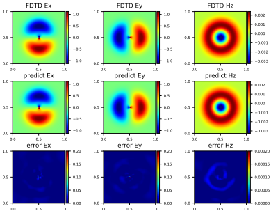
The instantaneous electromagnetic fields at the time of 2.4ns are showed in Fig.4. We can see that the predicted electromagnetic fields by our method are almost indistinguishable from the reference solution. The SIREN architecture (# subnets = 1) and our MS-SIREN architecture are used to solve the Maxwell's equations with a point source under different settings, and the final L2 errors of all output components and their mean values are shown in Table 1. It is obvious that MS-SIREN outperforms SIREN under all settings, and the best performance is achieved by the architecture comprising four subnets.
In order to approximate the Dirac delta function, the setting of kernel width α is important. In our experiments we find that the training process may not converge if α is too large or too small. We adopt an online fine-tuning method to decrease the value of α gradually during the training, which is illustrated in Fig.5 where the Gaussian distribution is used. The training process starts with α = 0.01, the L2 error drops rapidly and after 140k iterations the final mean L2 error is stable below 0.05. Then the online fine-tuning is performed to reduce the value of α by half, which makes the L2 error rise first but then decrease quickly as the training progresses, and after 70k iterations the final mean L2 error is stable below 0.08. The fine-tuning operation repeats twice that reduces the value of α to 0.0025 and 0.00125, respectively. According to the experimental results in Fig.5, we choose α = 0.01 as the kernel width and fix it in the other experiments. We further use Cauchy distribution and Laplacian distribution with α = 0.01 to approximate the point source, and get the final mean L2 errors as 0.04 and 0.05, respectively. This set of experiments demonstrate that approximating the Dirac delta function with a symmetric unimodal continuous probability density function is feasible.
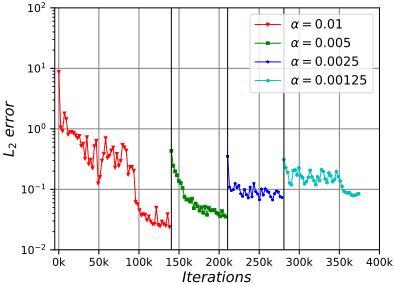
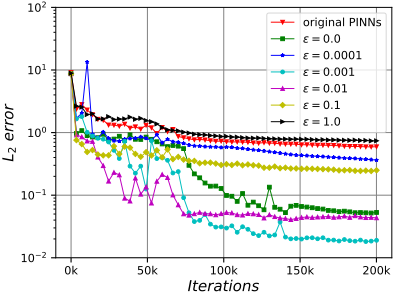
Fig.6 shows the L2 errors when different ϵ in Eq.(9) is used in solving Maxwell's equations with a point source. When ϵ = 0.01 and ϵ = 0.001, the lower bound constrained uncertainty weighting method outperforms the original uncertainty weighting method (ϵ = 0) with not only lower final L2 errors, but also faster convergence speed.
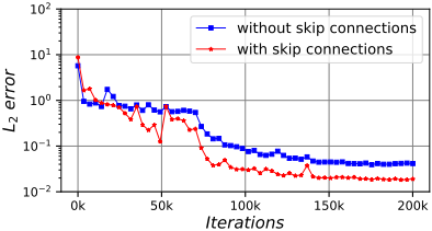
The MS-SIREN architecture uses skip connections between consecutive hidden layers. To validate its effectiveness, we compare MS-SIREN architectures with and without skip connections, and show the results in Fig.7. It is clear that skip connections make L2 error decrease faster and reach a lower value.
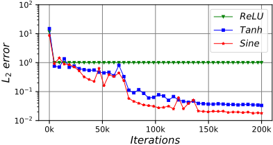
Activation function is another key factor affecting the prediction accuracy. To validate the effectiveness of Sine periodic activation function, we compare it with ReLU and Tanh, and the results are shown in Fig.8. Sine produces the best results in terms of convergence speed and the final mean L2 error. In comparison, Tanh performs slightly worse than Sine, and ReLU fails to let the network learn any useful information.
4.2 Poisson's Equation with a Point Source
We apply our approach to solve Eq.(2) in the region of Ω = [0, π] × [0, π] with the point source located at x0 = ( π2 , π2 ). The point source is approximated using Gaussian distribution with fixed α = 0.01 and the lower bound hyperparameter ϵ is set to 0.01.
Table 2 shows the prediction accuracy obtained by different network architectures. The SIREN architecture (# subnets =
1) cannot converge in all settings due to the singularity problem. However, when the number of subnets increases to 2 or 4, the L2 error drops remarkably. This experiment indicates that a multi-scale structure is necessary to solve this problem.
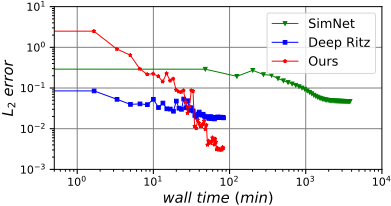
For comparison, we also apply Deep Ritz method and SimNet variational method to solve the problem. Fig.9 shows that the convergence speed of our method is close to that of Deep Ritz method, but faster than that of SimNet. The final L2 error obtained by our method is 0.003, which is significantly better than Deep Ritz (0.018) and SimNet (0.047). Moreover, our method is a more general approach that is not limited by the type of PDEs, whereas the Deep Ritz method and SimNet variational methods are the opposite.
4.3 Barry andMercer's Source Problem
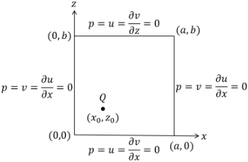
The third problem we solve is the nondimensionalized poroelastic Barry and Mercer's source problem with timedependent fluid injection. The governing equations are given by
where u and v are the deformations of porous medium along the x and z directions, p is the pore fluid pressure, Q is a fluid source or sink term, η and β are nondimensional parameters which are functions of the real material parameters. An illustration of the problem is shown in Fig.10. An oscillating point source Q located at (x0, z0) in the rectangular domain [0, a] × [0, b] is given by:
where ω is the oscillation frequency. The parameters are set as follows: a = b = 1, t ∈ [0, 2π], β = 2, η = 1.5, (x0, z0) = (0.25, 0.25) and ω = 1.
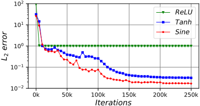
Table 3 shows the L2 errors achieved by different network architectures. Compared with the SIREN architecture (# subnets = 1), MS-SIREN does not bring any benefit in this case as the point source in this problem contains only one frequency component, and thus there are not multiple frequency components in the analytical solution. Fig.11 compares the convergence process with different activation functions. The periodic activation function Sine exhibits superior performance over ReLU and Tanh. In addition to Gaussian distribution, we also use Cauchy distribution and Laplacian distribution to approximate the Dirac delta function, and obtain L2 error being 0.051 and 0.025, respectively.
| Network Architectures | L2 error | |||||
|---|---|---|---|---|---|---|
| # subnets | # layers | # neurons | u | v | p | mean |
| 1 | 5 | 256 | 0.022 | 0.021 | 0.026 | 0.023 |
| 1 | 7 | 256 | 0.011 | 0.016 | 0.026 | 0.018 |
| 2 | 5 | 128 | 0.010 | 0.011 | 0.026 | 0.016 |
| 2 | 7 | 128 | 0.012 | 0.013 | 0.026 | 0.017 |
| 4 | 5 | 64 | 0.012 | 0.013 | 0.026 | 0.017 |
| 4 | 7 | 64 | 0.018 | 0.014 | 0.026 | 0.019 |
5 Conclusions
PDEs with a point source pose a great challenge to conventional PINNs method due to the singularity problem, and all the methods trying to tackle this problem so far can only work under certain constraints. We propose a universal approach based on the PINNs method that can solve the PDEs with a point source without any specific assumptions. The novelty of our approach lies in three aspects, approximating the Dirac delta function with a symmetric unimodal continuous probability density function, balancing the training loss terms of different areas with a lower bound constrained uncertainty weighting algorithm, and using multi-scale DNN with Sine activation function to build the network architecture. Three representative physical problems are used to verify the effectiveness of our method, and these experiments show that our method outperforms existing deep learning-based methods in accuracy, efficiency and versatility.
Acknowledgments
This work was supported by National Key R&D Program of China under Grant No. 2021ZD0110400.
@inproceedings{ijcai2022p533,
  title     = {A Universal PINNs Method for Solving Partial Differential Equations with a Point Source},
  author    = {Huang, Xiang and Liu, Hongsheng and Shi, Beiji and Wang, Zidong and Yang, Kang and Li, Yang and Wang, Min and Chu, Haotian and Zhou, Jing and Yu, Fan and Hua, Bei and Dong, Bin and Chen, Lei},
  booktitle = {Proceedings of the Thirty-First International Joint Conference on
               Artificial Intelligence, {IJCAI-22}},
  publisher = {International Joint Conferences on Artificial Intelligence Organization},
  editor    = {Luc De Raedt},
  pages     = {3839--3846},
  year      = {2022},
  month     = {7},
  note      = {Main Track},
  doi       = {10.24963/ijcai.2022/533},
  url       = {https://doi.org/10.24963/ijcai.2022/533},
}
TY - CPAPER TI - A Universal PINNs Method for Solving Partial Differential Equations with a Point Source AU - Huang, Xiang AU - Liu, Hongsheng AU - Shi, Beiji AU - Wang, Zidong AU - Yang, Kang AU - Li, Yang AU - Wang, Min AU - Chu, Haotian AU - Zhou, Jing AU - Yu, Fan AU - Hua, Bei AU - Dong, Bin AU - Chen, Lei T2 - Proceedings of the Thirty-First International Joint Conference on Artificial Intelligence, IJCAI-22 PB - International Joint Conferences on Artificial Intelligence Organization PY - 2022 SP - 3839 EP - 3846 DO - 10.24963/ijcai.2022/533 UR - https://doi.org/10.24963/ijcai.2022/533 ER -Copied
Machine-readable versions of this paper, for tools and AI agents:





