
Robustness Guarantees for Credal Bayesian Networks via Constraint Relaxation over Probabilistic Circuits
Proceedings of the Thirty-First International Joint Conference on Artificial Intelligence. Main Track. Pages 4885-4892.
https://doi.org/10.24963/ijcai.2022/677
Keywords
- Agent-based and Multi-agent Systems: Formal Verification, Validation and Synthesis
- AI Ethics, Trust, Fairness: Safety & Robustness
- Uncertainty in AI: Bayesian Networks
- Constraint Satisfaction and Optimization: Constraint Satisfaction
- Uncertainty in AI: Tractable Probabilistic Models
Abstract
In many domains, worst-case guarantees on the performance (e.g. prediction accuracy) of a decision function subject to distributional shifts and uncertainty about the environment are crucial. In this work we develop a method to quantify the robustness of decision functions with respect to credal Bayesian networks, formal parametric models of the environment where uncertainty is expressed through credal sets on the parameters. In particular, we address the maximum marginal probability (MARmax) problem, that is, determining the greatest probability of an event (such as misclassification) obtainable for parameters in the credal set. We develop a method to faithfully transfer the problem into a constrained optimization problem on a probabilistic circuit. By performing a simple constraint relaxation, we show how to obtain a guaranteed upper bound on MARmax in linear time in the size of the circuit. We further theoretically characterize this constraint relaxation in terms of the original Bayesian network structure, which yields insight into the tightness of the bound. We implement the method and provide experimental evidence that the upper bound is often near tight and demonstrates improved scalability compared to other methods.
- [Antonucci et al., 2010] Alessandro Antonucci, Yi Sun, Cas- sio P. de Campos, and Marco Zaffalon. Generalized loopy 2u: A new algorithm for approximate inference in credal networks. Int. J. Approx. Reasoning, 51(5):474-484, jun 2010.
- [Antonucci et al., 2015] Alessandro Antonucci, Cassio P. de Campos, David Huber, and Marco Zaffalon. Approximate credal network updating by linear programming with ap- plications to decision making. Int. J. Approx. Reasoning, 58:25-38, 2015.
- [Cabañas and Antonucci, 2021] Rafael Cabañas and Alessandro Antonucci. Crepo: An open repository to benchmark credal network algorithms. arXiv preprint arXiv:2105.04158, 2021.
- [Cano et al., 2007] Andrés Cano, Manuel Gómez, Serafín Moral, and Joaquín Abellán. Hill-climbing and branch- and-bound algorithms for exact and approximate inference in credal networks. Int. J. Approx. Reasoning, 44(3):261- 280, 2007. Reasoning with Imprecise Probabilities.
- [Chan and Darwiche, 2004] Hei Chan and Adnan Darwiche. Sensitivity analysis in bayesian networks: From single to multiple parameters. In UAI, page 67-75, Arlington, Vir- ginia, USA, 2004. AUAI Press.
- [Chan and Darwiche, 2006] Hei Chan and Adnan Darwiche. On the robustness of most probable explanations. In UAI, page 63-71, July 2006.
- [Coupé et al., 2000] Veerle M. H. Coupé, Linda C. Van Der Gaag, and J. Dik F. Habbema. Sensitivity analysis: An aid for belief-network quantification. Knowl. Eng. Rev., 15(3):215-232, sep 2000.
- [Cozman, 2000] Fabio G. Cozman. Credal networks. Artifi- cial Intelligence, 120(2):199-233, 2000.
- [Darwiche, 2003] Adnan Darwiche. A differential approach to inference in bayesian networks. Journal of the ACM (JACM), 50(3):280-305, 2003.
- [De Campos and Cozman, 2007] Cassio Polpo De Campos and Fabio Gagliardi Cozman. Inference in credal networks through integer programming. In Proceedings of the Fifth International Symposium on Imprecise Probability: Theo- ries andApplications, 2007.
- [Fagiuoli and Zaffalon, 1998] Enrico Fagiuoli and Marco Zaffalon. 2u: An exact interval propagation algo- rithm for polytrees with binary variables. Artif. Intell., 106(1):77-107, nov 1998.
- [Huber et al., 2020] D. Huber, R. Cabañas, A. Antonucci, and M. Zaffalon. CREMA: a Java library for credal net- work inference. In M. Jaeger and T.D. Nielsen, editors, Proceedings of the 10th International Conference on Prob- abilistic Graphical Models (PGM 2020), Proceedings of Machine Learning Research, Aalborg, Denmark, 2020. PMLR.
- [Katz et al., 2017] Guy Katz, Clark Barrett, David L Dill, Kyle Julian, and Mykel J Kochenderfer. Reluplex: An efficient smt solver for verifying deep neural networks. In CAV, pages 97-117. Springer, 2017.
- [Lipton et al., 2018] Zachary Lipton, Yu-Xiang Wang, and Alexander Smola. Detecting and correcting for label shift with black box predictors. In ICML, pages 3122-3130.
- PMLR, 2018.
- [Mattei et al., 2020] Lilith Mattei, Alessandro Antonucci, Denis Deratani Mauá, Alessandro Facchini, and Julissa Villanueva Llerena. Tractable inference in credal sentential decision diagrams. International Journal of Approximate Reasoning, 125:26-48, 2020.
- [Mauá et al., 2017] Denis D Mauá, Fabio G Cozman, Diar- maid Conaty, and Cassio P Campos. Credal sum-product networks. In Proceedings of the Tenth International Sym- posium on Imprecise Probability: Theories and Applica- tions, pages 205-216. PMLR, 2017.
- [Mauá and Cozman, 2020] Denis Deratani Mauá and Fabio Gagliardi Cozman. Thirty years of credal networks: Specification, algorithms and complexity. Int. J. Approx. Reasoning, 126:133-157, 2020.
- [Narodytska et al., 2018] Nina Narodytska, Shiva Ka- siviswanathan, Leonid Ryzhyk, Mooly Sagiv, and Toby Walsh. Verifying properties of binarized deep neural networks. In AAAI, volume 32, 2018.
- [Pearl, 1985] Judea Pearl. Bayesian networks: A model of self-activated memory for evidential reasoning. In Pro- ceedings of the 7th conference of the Cognitive Science Society, University of California, Irvine, CA, USA, pages 15-17, 1985.
- [Poon and Domingos, 2011] Hoifung Poon and Pedro Domingos. Sum-product networks: A new deep architec- ture. In UAI, page 337-346, July 2011.
- [Quiñonero-Candela et al., 2009] Joaquin Quiñonero- Candela, Masashi Sugiyama, Neil D Lawrence, and Anton Schwaighofer. Dataset shift in machine learning. Mit Press, 2009.
- [Rooshenas and Lowd, 2014] Amirmohammad Rooshenas and Daniel Lowd. Learning sum-product networks with direct and indirect variable interactions. In ICML, pages 710-718. PMLR, 2014.
- [Ruan et al., 2018] Wenjie Ruan, Xiaowei Huang, and Marta Kwiatkowska. Reachability analysis of deep neural net- works with provable guarantees. In IJCAI, IJCAI'18, page 2651-2659. AAAI Press, 2018. IJCAI
- [Wang et al., 2021] Benjie Wang, Clare Lyle, and Marta Kwiatkowska. Provable guarantees on the robustness of decision rules to causal interventions. In IJCAI, 2021. IJCAI
- [Zaffalon et al., 2020] Marco Zaffalon, Alessandro An- tonucci, and Rafael Cabañas. Structural causal models are (solvable by) credal networks. In International Confer- ence on Probabilistic Graphical Models, pages 581-592.
- PMLR, 2020.
- [Zhang et al., 2015] Kun Zhang, Mingming Gong, and Bern- hard Schölkopf. Multi-source domain adaptation: A causal view. In AAAI, 2015.
References were extracted automatically from the PDF and may contain errors.
Full text extracted automatically from the PDF; figures, tables and equations may differ. The PDF is the version of record.
1 Introduction
Probabilistic models allow us to make quantitative inferences about the behaviour of complex systems, and are an important tool to guide their use and design. When such models are learnt from data, exposed to potential distribution shifts or are partially unknown, it is important to be able to verify the robustness of inferences on the model to these uncertainties. This is particularly relevant for decision functions taking action in the model, where much work has gone into verifying worst-case behaviour when exposed to various disturbances or changes in the environment (distribution shifts). Causal Bayesian networks (BNs) [Pearl, 1985] are compelling models for this purpose, since one can perform causal interventions on them, giving rise to families of distributions that share a common structure. However, performing useful inference on BNs is often intractable, and one way to address this is to compile them into more tractable representations such as arithmetic circuits [Darwiche, 2003]. Recent work has shown that such compilation methods can also efficiently compute bounds on a decision function's robustness to causal interventions [Wang et al., 2021]. A limiting factor on the applicability of these methods is the need to have an exact model, where all non-intervened parameters are known precisely. This is difficult to achieve when learning parameters from data, since most settings will only allow reliable determination up to some error bound ϵ.
In this paper we study robustness of credal Bayesian networks (CrBNs) [Mau´a and Cozman, 2020], a generalisation of Bayesian networks where parameters are only known to be within some credal sets (e.g., intervals). They can be used to model causal interventions, but are also very well suited to modelling parameters learned from data, as well as modelling of exogenous variables [Zaffalon et al., 2020].
We consider the maximum marginal probability (MARmax) problem for CrBNs and develop a solution by encoding the network as a tractable probabilistic circuit (a credal extension of sum-product networks, called CSPNs). More specifically, this paper makes the following contributions: (i) a method for constructing a probabilistic circuit whose parameters represent the conditional probability distributions of a BN, allowing the transfer of credal inference problems from a highly intractable setting (CrBNs) to a tractable one (CSPN) through constraint relaxation; (ii) algorithms which make use of this transfer to compute upper and lower bounds on probabilities of events under many forms of parameter uncertainty; (iii) a characterization of the tightness of the upper bound in terms of the network structure; and (iv) an empirical evaluation demonstrating comparable precision and significantly improved scalability compared to state-of-the-art credal network inference, while also providing formal guarantees.
Some details and proofs can be found in the Appendix at http://www.fun2model.org/bibitem.php?key=WWK22
1.1 RelatedWork
The problem of robustness of inferences under imprecise knowledge of the distribution has been studied under many guises. In the machine learning community, there has been much work on robustness of classifiers to simple adversarial attacks or distribution shifts [Qui ˜nonero-Candela et al., 2009; Zhang et al., 2015; Lipton et al., 2018]. Motivated by safety concerns, methods have been developed to compute formal guarantees of robustness through constraint solving [Katz et al., 2017; Narodytska et al., 2018] or output reachability analysis [Ruan et al., 2018]. However, these methods do not model the environment, and are thus limited in the types of distributional shifts they can address.
In the Bayesian network literature, robustness has primarily been studied in terms of the effect of parameters on inference queries, such as marginal probabilities. For instance, sensitivity analysis [Coup´e et al., 2000; Chan and Darwiche, 2004] is concerned with the effect of small, local changes/perturbations to parameters. Closer to our work is the formalism of credal networks [Mau´a and Cozman, 2020], which represent imprecise knowledge by positing sets of parameters for each conditional distribution, rather than precise values. Inference then corresponds to computing maximal (or minimal) probabilities over the possible parameter values. Unfortunately, exact methods for inference in credal networks do not perform well except for smaller networks with simple credal sets, or in special cases such as polytrees [Fagiuoli and Zaffalon, 1998; De Campos and Cozman, 2007]. On the other hand, approximate methods [Cano et al., 2007; Antonucci et al., 2010; Antonucci et al., 2015] usually cannot provide theoretical guarantees (upper bounds), limiting their applicability in safety-critical scenarios.
This paper builds on work showing the tractability of credal inference for certain probabilistic circuits [Mau´a et al., 2017] [Mattei et al., 2020]. Our key contribution is a method for mapping credal network problems into tractable inference problems on such probabilistic circuits, which affords not only greater scalability compared to the state-of-the-art in credal network inference, but also formal guarantees.
Finally, methods for providing robustness guarantees for classifiers in combination with a Bayesian network environment model have recently been proposed [Wang et al., 2021]. Our paper generalizes and extends their work, enabling efficient computation for broader and more realistic classes of parameter uncertainty.
2 Background
A Bayesian network (BN) N = (G,Θ) over discrete variables V = {V1, ..., Vn} consists of a directed acyclic graph (DAG) G = (V ,E) and a set of parameters Θ. It is a factoring of a joint probability distribution pN into conditional distributions for each variable, such that
where the parents pa(Vi) of Vi are the set of variables Vj such that (Vj, Vi) ∈ E. Θ is the set of parameters of the form:
for each instantiation vi, ui of a variable Vi and parents Ui.
Given a Bayesian network model, to obtain useful information about the distribution we will need to perform inference. For example, we might wish to obtain the probability pN(W = w) for some subset of variables W ⊆ V , a procedure known as marginalization. In the worst case, marginal inference in Bayesian networks is known to be #P-complete, though many practical inference methods exist.
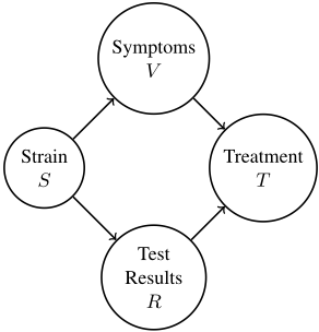
Given a classifier, we can represent its input-output behaviour using a decision function F : X → Y , which observes some subset X ⊆ V and tries to predict Y ∈ V . To combine this with a Bayesian network environment model N, we follow [Wang et al., 2021] in the construction of an augmented BN NF , which is a Bayesian network based on N where an additional variable (node) ˆ Y is added with pa( ˆ Y ) = X and pNF ( ˆ Y = ˆ y|X = x) = 1[ˆ y = F(x)]. NF is thus a unified model of environment and decision maker, and inference on the model can answer questions such as the prediction accuracy pNF ( ˆ Y = Y ).
3 Robust Inference on Bayesian Networks
It is rarely the case that we can specify the parameters of a Bayesian network with complete certainty before performing inference. Firstly, whether the parameters are learned from data or elicited from expert knowledge, the knowledge that we obtain regarding the parameters is typically imprecise, specified as sets or intervals. Secondly, when the Bayesian network is imbued with a causal interpretation, one is often concerned about potential distribution shift, modelled by causal interventions, and their effect on inference queries.
As a running example, consider a fictional scenario depicted in Figure 1, where patients are infected by some unobservable strain S of a disease, with some strains much more severe than others, and a decision rule F must be created based on observable symptoms V and test results R that decides whether to administer an expensive treatment option. While it is desirable to save resources by only administering treatment for the more severe strains, , a guarantee is needed that the decision rule has a robustly low probability of not treating a severe case. To provide such a guarantee we model the system as an augmented BN NF over variables {S, V,R, T}, where T is binary and deterministic, given by F (v, r). However, we do not have precise knowledge over the parameters of the BN, so we instead design intervals which specify the range of values a parameter could take.
We start with θS, the distribution over the strains. We expect that the decision rule will be deployed across a variety of areas and times, and as such we are concerned about distributional shifts in θS. We could thus decide to allow any probability distribution across the strains, i.e. θS=s ∈ [0, 1]. We imagine the tests used are very well understood, and we know θR|s exactly. Moving onto the parameters θV |s, describing the symptoms of a particular strain, we might expect that these, unlike θS, are relatively fixed across different settings. However, gathering enough data on each strain and symptom combination to be certain of this (fixed) parameter value might turn out to be challenging. In this case it might be suitable to take mean estimates of the parameter values θ∗V =v|s , and then select some confidence interval [θ∗V =v|s - ϵ, θ∗V =v|s + ϵ].
3.1 Credal Bayesian Networks
We can model this using credal Bayesian networks [Mau´a and Cozman, 2020], a framework that encompasses both causal interventions and imprecise knowledge of parameters.
Definition 1. Let pΘ,Θ ∈ Θ, be any parameterised probability distribution, where Θ is the set of allowed parameter values. Then we call C ⊆ Θ a credal set for this parameterisation, and the credal family Cp[C] = {pΘ′ |Θ′ ∈ C} is the family of distributions where the parameters are in C.
This is a maximally expressive formalism for credal uncertainty. However, an independence assumption between the uncertainty of different conditional distributions in a BN (sometimes known as the strong extension [Cozman, 2000]) is usually assumed:
Definition 2. [Cozman, 2000] A Credal BN (CrBN) CN [C] = {NΘ |Θ ∈ C} over a BN NΘ = (G, Θ) is a credal family satisfying
i.e. the credal set decomposes as a cartesian product of separate credal sets for each variable Vi and instantiation of its parent variables ui.
Since augmented Bayesian networks are simply Bayesian networks with an additional deterministic node (the decision function), we can convert any credal set over a Bayesian network model N to a credal set over NF by maintaining the credal sets for all variables, while assuming the conditional distribution for the new variable ˆ Y is known exactly. This framework then fully generalizes the "interventional robustness problem" introduced by [Wang et al., 2021] to allow arbitrary credal sets for parameters; see Appendix for details.
3.2 ProblemDefinition
In the treatment example we wished to guarantee the worstcase probability of an event occurring over a CrBN. We will now formalise this problem.
Definition 3. Given an (augmented) CrBN CN [C]
and an event e (an instantiation of a subset of the variables), the maximum marginal probability (MARmax) problem is that of determining
| s1 | s2 | s3 | |
|---|---|---|---|
| θR | 0.95 | 0.05 | 0.5 |
| θV | 0.2±0.1 | 0.8±0.1 | 0.6±0.2 |
This generalization of causal interventions enables many new problems to be considered, as causal interventions require parameters to be known exactly or be entirely unknown. Crucially, it allows us to model parameters which are estimated from data to be within some interval. It also allows the degree of uncertainty to depend on the value of the parents, as it might if some parent values are rare and lack data points.
As an illustration we now define a CrBN over NF to formalize the treatment scenario in Figure 1. We imagine there are three strains s1, s2, s3, of which only s3 is severe and requires treatment. We take V and R to be binary variables (symptomatic/asymptomatic and positive/negative test). We wish to be able to apply the decision rule in any situation where the prevalence of s3 is at most 0.1, so we assign CS = {θ ∈ Z3|θS=s3 < 0.1}, where Z3 is the threedimensional probability simplex. We use singleton credal sets for R and confidence intervals for V , with the values given in Table 1. The decision rule to be analysed gives treatment when R = V , since this is unlikely for s1 and s2.
This is an instance of the maximum marginal probability MARmax problem, where the CrBN CN[C] is as specified above, and the event of interest is e = (T = 0) ∧ (S = s3).
4 Credal Robustness via Probabilistic Circuits
In this section, we present an efficient method for bounding MARmax credal robustness for Bayesian networks with guarantees. In particular, the method returns an upper bound on MARmax. In the treatment example, this would mean that we can be certain that the probability of denying treatment to a patient with the severe strain does not exceed the computed value, assuming all parameters lie within the credal sets. Our method is based upon establishing a correspondence between credal BNs and credal sum-product networks (CSPN) [Mau´a et al., 2017], a recently proposed model which introduces uncertainty sets over the weights of a sum-product network. In particular, we develop an algorithm for compiling CrBNs into equivalent CSPNs. By efficiently solving a similar credal maximization problem on the CSPN, we can derive upper bounds on MARmax for the original CrBN.
4.1 Compilation to Arithmetic Circuits
The first step of our method is to compile the credal Bayesian network to an arithmetic circuit. To describe this, we first consider an alternative representation of a Bayesian network.
Definition 4. [Darwiche, 2003] The network polynomial of a BN N is defined as
where λvi are indicator variables for variable Vi, which take the value 1 if Vi = vi and 0 otherwise.
The network polynomial is a multilinear function which unambigously encodes the graphical structure of the Bayesian network, for any value of the parameters Θ. In particular, one can obtain the joint probability pN(v1, ..., vn) for any instantiation v1, ..., vn by setting the indicator variables and evaluating the network polynomial. Unfortunately, it has an exponential number of terms in the number of variables of the BN, which means we cannot use it directly. The goal of compilation is to represent the network polynomial more efficiently, by exchanging sums and products where possible. The result of such a procedure can be interpreted as a rooted directed acyclic graph (DAG) called an arithmetic circuit.
Definition 5. [Darwiche, 2003] An arithmetic circuit (AC) T over variables V and parameters Θ is a rooted DAG, whose internal nodes are labelled with + or × and whose leaf nodes are labelled with indicator variables λv
or non-negative parameters. For an internal node t we will write Tt for the arithmetic circuit containing t and all its descendants.
Definition 6. [Chan andDarwiche, 2006] A complete subcircuit α of an AC is obtained by traversing the circuit top-down, choosing one child of every visited +-node and all children of every visited ×-node. The term term(α) of α is the product of all leaf nodes visited (i.e. all indicator and parameter variables). The AC polynomial lT [λ,Θ] is the sum of the terms of all complete subcircuits.
Compilation will produce an AC T which has the same polynomial as the BN, i.e. lN[λ,Θ] = lT [λ,Θ]. In addition, it will satisfy technical conditions called decomposability, determinism and smoothness, which allow us to perform many inference queries in linear time in the size of the circuit.
In [Wang et al., 2021] a method is described for compiling an augmented BN to a smooth, decomposable and deterministic AC, which allows one to tractably compute marginal probabilities involving both the decision function and Bayesian network variables. In order to support further queries, they additionally impose ordering constraints on the AC.
Definition 7. A +-node t with children t1, ..., tn in an arithmetic circuit T splits on variable Vi if there exists an ordering of the domain v1 i , ..., vn i of Vi such that all complete subcircuits of Tti contain the indicator λvi .
Definition 8. Let σ = (V1, ..., Vn) be a topological ordering of the variables in BN N. We say that an (smooth, decomposable, deterministic) arithmetic circuit T computes the BN N respecting σ if:
- lT [λ,Θ] = lN[λ,Θ]
- Each +-node in T splits on some variable Vi. We define split(t) for a +-node t to be the variable it splits on.
- The variables are split respecting the topological order. That is, if Vi = split(t), Vj = split(t′ ), then
In other words, it is required that the AC represents the same polynomial as the BN, and further that the AC satisfies particular structural constraints that mean that the AC must split on parents before children. This leads to the following new result, which intuitively means that, when an AC splits on variable V , the values of its parents are already known.
Lemma 1. Suppose that T computes N respecting some topological order. Let t be a +-node in T splitting on some variable V . Then all complete subcircuits α which include t must agree on the value of its parents paN (V ).
The AC compiled from the treatment example (Figure 1) is too large to include in its entirety, but Figure 2a shows one branch from the root sum node, with +-nodes labelled with the variable they split on. Notice that the topological order (S, R, V, T ) is respected, and that, at every +-node, the value of the parents of the splitting variable are already "known".
4.2 Compiling to Credal SPNs
While this compiled AC allows us to efficiently compute marginals for given parameter values Θ, it does not effectively represent credal sets, and thus finding maximizing parameter values is challenging (one would need to solve constraints potentially spread out across the whole circuit).
In the next step of our method, we further compile the AC to a sum-product network (SPN). SPNs differ from ACs in that they lack parameter nodes and instead have parameters (i.e. weights) associated with branches from sum nodes.
Definition 9. [Poon and Domingos, 2011] A sum-product network (SPN) over variables V and with weights W is a rooted DAG whose internal nodes are labelled with either + or ×, and whose leaf nodes are labelled with indicator variables λv. The branches of a sum node ti with k branches are labelled with weights wi,1, .., wi,k.
Definition 10. A complete subcircuit α of an SPN S is obtained by traversing the circuit top-down, choosing one child of every visited +-node and all children of every visited ×- node. The term term(α) of α is the product of all leaf nodes visited (i.e. all indicators) and all weights wij along branches chosen by the subcircuit.
The SPN-polynomial lS[λ,W] is the sum of the terms of all complete subcircuits.
Our compilation differs from that presented in [Rooshenas and Lowd, 2014] in that we make use of the particular structure of the AC, shown in Lemma 1, to make sure the weights on the sum nodes directly correspond to the parameters in the BN (which would not be the case under standard compilation).
At a high level, the compilation only involves two steps:
- For each sum node t splitting on Vi, assign weights over branches according to θVi|ui , where all variables in ui are known due to Lemma 1.
- Remove all parameter nodes.
To algorithmically decide which parameters correspond to a particular sum node we construct a notion of 'possible values' for variables at nodes in the SPN. We first say that a node 'conditions' on V = v if the node is a parameter node θW=w|V=v,U=u, and define
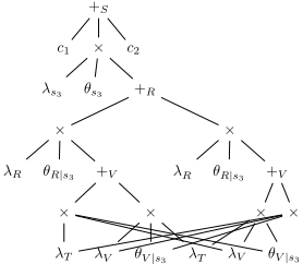
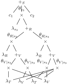
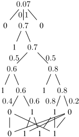
Figure 2: Illustration of Algorithm 2 for the treatment example. Due to space constraints we show only the S = s3 branch of the AC/SPN.
Corollary 1. For any sum node t splitting on V , if W is a parent of V then Pt(W) must contain exactly one possible value.
Proof. Any complete subcircuit corresponds to a term of the network polynomial, and must contain a parameter θV |wi,ui for some wi, ui. This parameter cannot occur as an ancestor of t, since it would then be impossible to satisfy Definition 7, and so it must be a descendant. Thus Pt(V ) is non-empty. By Lemma 1, it cannot contain more than 1 element.
These sets uniquely determine the values of all parents, and thus which parameters to use. The sets can be efficiently computed , as described in Algorithm 1.
Figure 2b shows the result for the AC in Figure 2a.
Algorithm 1: SPN compilation from AC
Input: AC T computing N and satisfying Definition 8.
Result: An SPN computing N where all sum node weights correspond to a CPT θVi|ui
1 begin
- 2 For indicator nodes t, assign Pt(V ) = {}; 3 For parameter nodes θv|u1,u2,...,, assign Pt(Ui) = {ui} if Ui ∈ pa(V ) and Pt(Ui) = {} otherwise;
- 4 For inner nodes t compute Pt(V ) = ⋃c∈children(t) Pc(V );
- 5 For sum nodes t, label the edges according to θV |u1,u2,..., where t splits on V and ui is the unique value in Pt(Ui);
- 6 Remove all parameter nodes.
Proposition 1. Given an arithmetic circuit T which computes N satsifying some topological order, the SPN S compiled as above satisfies
Proof. We can put the complete subcircuits of T and S in a one-to-one correspondence by the choice of branch at each sum node (since only the parameter nodes/weights have changed). Let αT be a subcircuit of T , and αS the corresponding subcircuit of S. For every variable V , αT contains exactly one +-node splitting on V , and exactly one parameter of the form θV |pa(V ). The compilation procedure moves this parameter to be a weight of the +-node splitting on V , so that the overall term is unchanged. Applying this to all variables, we have that term(αT ) = term(αS), and thus the result.
For credal families over SPNs satisfying an independence requirement between all sum nodes (such that knowing the weights of one sum node does not affect your uncertainty over other weights), MARmax can be computed efficiently. These are exactly the Credal SPNs introduced in [Mau´a et al., 2017].
Definition 11. [Mau´a et al., 2017] A Credal SPN (CSPN) is a credal family CS[C] over an SPN S satisfying
where Ci is a subset of a probability simplex on the weights of sum node i.
We can construct a credal family over the compiled SPN, which is equivalent to our CrBN, by requiring all sum nodes that split on a variable Vi and have parents ui to (i) all have the same weights and (ii) have that weight be in CVi|ui . However, this will not in general be a CSPN, since (i) breaks the independence requirement (observing the weights of one sum node will change the credal set for a different sum node if they both split on the same variable with the same values of the parents).
We can, however, construct a CSPN by removing requirement (i), which creates a strictly larger credal family. This relaxation is the final step of our compilation process.
Lemma 2. For a CrBN CN[CN] and its compiled CSPN CS [CS ],
Proof. For any given Θ ∈ CN we have lS[λ, Θ] = lN [Θ, λ], by Proposition 1 and the fact that S computes N. The only way to violate the inequality is if Θ /∈ CS. But CS only demands that at each sum node t splitting on Vi the parameters are in CVi|ui , which will certainly be true if Θ ∈ CN .
If we apply this to construct a CSPN for our treatment example, it will be a CSPN over the SPN in Figure 2b, where the weights of the sum nodes are constrained by the credal sets of the CrBN defined in Section 3.2.
4.3 Solving MARmax
Analogously to CrBNs, we can define the maximum marginal probability problem for CSPNs as MARmax(S, C, e) = maxΘ∈C lS[λe, Θ], where λe refers to the appropriate instantiation of the indicators for the event e.
While MARmax for the AC (and BN) is intractable, we can compute it efficiently for a CSPN [Mau´a et al., 2017].
Proposition 2. Given a Credal SPN CS[∏ni=1 Ci], we can solve MARmax for this family of distributions in O(|S|L), where L is an upper bound on solving maxwi ∑j wijcj subject to wi ∈ Ci.
Proof. If we assume the maximum possible value of the children c1, ..., cj of a sum node ti are known, finding the maximum possible value of ti can be done by solving maxwi ∑j wijcj subject to wi ∈ Ci. The same is true for product nodes, with the maximum value being the product of the maximum values of its children. By induction we can find the maximum possible value of the root node through bottomup evaluation. For details see [Mau´a et al., 2017].
Figure 2c illustrates the computation on the CSPN compiled from the treatment example. The algorithm evaluates nodes bottom up in the graph, with the indicators set to their appropriate value (λT = λs1 = λs2 = 0, the rest 1). The s1, s2 branches always lead to an indicator with the value 0. When a sum node is reached, the maximizing weights allowed by the credal set at that sum node are picked. For the left +V node this means assigning θV |s3 the lowest weight allowed (0.4), while the right +V is instead maximized with the highest weight allowed (0.8). No choice is made at +R since it is a singleton, and at +S the maximumweight for s3 (0.1) is chosen. This demonstrates that MARmax(S, C, ¯ T∧s3) = 0.07.
Our overall method CUB is summarized in Algorithm 2. The following theorem, which follows directly from Lemma 2, shows that we do indeed return an upper bound:
Algorithm 2: Upper Bounding for MARmax
Input: Credal Bayesian Network CN [CN ], event e, order σ
Result: Upper bound on MARmax(N , CN , e)
1 begin
- 2 Compile N to AC obeying topological order σ;
- 3 Construct a credal SPNCS[CS] from the AC;
- 4 Compute MARmax(S, CS, e) for this credal SPN;
- 5 Return MARmax(S, CS, e)
Theorem 2. The output MARmax(S, CS, e) returned by Algorithm 2 satisfies
Thus, we find that the probability of not assigning treatment to a patient with the severe strain in the treatment example can be no greater than MARmax(S, C, ¯ T ∧ s3) = 0.07.
4.4 Tightness of Upper Bound
Though our algorithm provides an upper bound on MARmax for the Bayesian network, it will not typically be tight. This is illustrated in Figure 2c, where the two different sum nodes representing θV |s3 are assigned different weights by the maximization in the CSPN, while this is not possible for the original CrBN. We will now provide a precise characterization of the looseness of the upper bound, using the concept of structural enrichment to find an enriched CrBN which can be put in a 1-1 correspondence with the CSPN.
Definition 12. A structural enrichment of a CrBN CN[C] is a new CrBN CN ′ [C′ ] with a new underlying graph (V , E′ ) such that E ⊆ E′ , and a new credal set given by
where Ui are the parents of Vi in N, while Wi are the newly added parents in N ′ which were not parents in N.
To illustrate this, suppose that we had a BN with 3 variables A, B, C, where A is the only parent of C and we have the credal set θC=0|A=0 ∈ [0.3, 0.8]. If we now consider a structurally enriched BN where A, B are both parents of C, then we have the same interval θC=0|A=0,B=b ∈ [0.3, 0.8] for b ∈ {0, 1}, but, crucially, the parameters for b = 0 and b = 1 can take different values in this interval.
Definition 13. Given a CrBN CN[C] and ordering σ, the maximal structural enrichment CN + σ [C+σ ] is the (unique) structurally enriched CrBN which has an edge (Vi, Vj) for all i <σ j.
The maximal structural enrichment of a CrBN with some ordering simply allows for the choice of parameters (within the credal set) at some variable to depend on all variables earlier in the order. In the case of the treatment example, the ordering S, R, V, T (used for compilation in Figure 2a) would give a structurally enriched CrBN where the parameter θV |s3 is allowed to depend on R, as it does in the CSPN (Figure 2c).
Theorem 3. The output MARmax(S, C, e) returned by Algorithm 2 using ordering σ satisfies
An implication of this result (see Appendix for the proof) is that the ordering σ used when compiling the SPN can affect the tightness of the bound. Consequently, it is possible to search over topological orderings to obtain a better bound, at the cost of additional computation; we exploit this in our experiments as the method MCUB. It also demonstrates that if we do, in fact, want to bound the probability of an event in a maximally ordered enrichment, then Algorithm 2 will give an exact result.
We can also make use of this result to lower bound MARmax. We can project the optimal parameters θ+ Vi |ui ,wi found for CN + σ [C+σ ] to obtain parameters θVi|ui = θ+ Vi |ui ,w∗ i valid for CN[C], by fixing some w∗ i for each credal set. It is not guaranteed that the exact solution for CN[C] will be such a projection, but it is much easier to search over projections than parameter values and this can provide a strong lower bound in many cases, or serve as a way to initialize a more thorough search algorithm. In our experiments we will evaluate a local greedy search algorithm CLB, which is initialized to an arbitrary projection given by some wi for each credal set Ci, and tries a series of local changes wi → w′i , keeping any that increase the probability. It terminates if it reaches parity with the upper bound or no local improvement can be found. Note that there is no guarantee of convergence to the upper bound - by Theorem 3 it is only possible when MARmax(N + σ , C+σ , e) = MARmax(N, C, e), and even when this holds CLB can get stuck in local optima.
5 Experimental Results
We evaluate our method on the CREPO [Caba˜nas and Antonucci, 2021] [Huber et al., 2020] credal inference benchmark, which consists of 960 queries over 377 small-tomoderately sized networks, and, to evaluate scalability, hepar2, a 70-node Bayesian network. We include three of our methods 1 : (i) CUB, which computes an upper bound; (ii) MCUB (minimal ordering credal upper bound), which searches over (n = 30) orderings to obtain a better bound; and (iii) CLB, which computes a lower bound as described in Section 4.4 (capped to n = 100 steps).
We compare the performance of our methods to exact credal variable elimination [Cozman, 2000] (where feasible) and ApproxLP [Antonucci et al., 2015], an approximate method returning a lower bound which has been shown to be state of the art both in terms of scalability and accuracy of inferences. We do not consider comparison to the IntRob algorithm presented in [Wang et al., 2021] as it cannot address arbitrary credal sets, and Algorithm 2 is equivalent to theirs in the limited cases where both can be applied (when all credal sets are either singletons or maximal).
We split CREPO into two subsets, CREPOe (768 queries), where an exact solution could be computed, and CREPOh (192 queries), of hard queries where it ran out of memory (16GB). Since other methods do not support inferences involving decision functions, we use an augmented BN only for hepar2, where both the exact and ApproxLP methods run out of memory even without a decision function.
In Table 2, for all benchmarks we report the time taken by each method. For CREPOe, we compute the average difference in computed probability to the exact result (positive/negative for upper/lower bounds respectively), while for the other sets we report the average difference to the best upper bound. Remarkably, we see that our upper-bounding and lower-bounding algorithms dominate ApproxLP on CREPOe, with better lower bounds being produced in an order of magnitude less time. Given the simplicity of the greedy iteration in CLB, this is primarily explained by the effectiveness of projection from the upper bound as a starting heuristic. On CREPOh, our upper bounding is the only method capable of providing guarantees. Meanwhile, our lower bound performs worse on average than ApproxLP, but only by a small amount, while using significantly less time. Finally, we see that our method is the only one to scale to the challenging hepar2 network, completing in a reasonable amount of time even with the significant additional computational expense of incorporating a decision function.
1 Code for algorithms and experiments available at https://github.com/HjalmarWijk/credal-bound
| Dataset | ApproxLP | CLB | MCUB | CUB | |
|---|---|---|---|---|---|
| CREPOe | Diff T(ms) | -0.052 | -0.043 | 0.0015 | 0.0018 8 |
| 384 | 52 | 827 | 0.022 | ||
| CREPOh | Diff T(ms) | -0.053 1154 | -0.074 71 | 0 849 | 8 |
| Diff | - | -0.092 | - | 0 | |
| Hepar2 | T(s) | - | 716 | - | 293 |
6 Conclusions
We have demonstrated how to construct an SPN whose parameters (sum node weights) can be semantically interpreted as representing specific conditional probability distributions in a CrBN. The result relies on a novel SPN compilation technique, which ensures that (i) all sum nodes correspond to some variable V and (ii) that the values of all parents of V can be uniquely determined. This is significant as (after applying constraint relaxation) it enables a direct mapping of the credal sets of the CrBN to a CSPN, which, unlike the CrBN, can be tractably maximized. This gives an efficient method to analyse robustness of decision functions learnt from data in the presence of imprecise knowledge, distributional shifts and exogenous variables. Our method provides formally guaranteed upper and lower bounds on the probability of an event of interest, and the experimental evaluation has additionally demonstrated that it compares favourably in accuracy to stateof-the-art approximate methods while being orders of magnitude faster.
In future work the upper bound could be improved through reintroducing some of the dropped equality constraints between weights of sum nodes in the CSPN, though this will involve trade-offs between computational challenge and accuracy. The methodology could also be extended to handle more challenging queries such as maximum expectations, by imposing additional structure on the compiled circuit.
Acknowledgements
This project was funded by the ERC under the European Union's Horizon 2020 research and innovation programme (FUN2MODEL, grant agreement No. 834115), and by the Future of Humanity Institute, Oxford University.
@inproceedings{ijcai2022p677,
  title     = {Robustness Guarantees for Credal Bayesian Networks via Constraint Relaxation over Probabilistic Circuits},
  author    = {Wijk, Hjalmar and Wang, Benjie and Kwiatkowska, Marta},
  booktitle = {Proceedings of the Thirty-First International Joint Conference on
               Artificial Intelligence, {IJCAI-22}},
  publisher = {International Joint Conferences on Artificial Intelligence Organization},
  editor    = {Luc De Raedt},
  pages     = {4885--4892},
  year      = {2022},
  month     = {7},
  note      = {Main Track},
  doi       = {10.24963/ijcai.2022/677},
  url       = {https://doi.org/10.24963/ijcai.2022/677},
}
TY - CPAPER TI - Robustness Guarantees for Credal Bayesian Networks via Constraint Relaxation over Probabilistic Circuits AU - Wijk, Hjalmar AU - Wang, Benjie AU - Kwiatkowska, Marta T2 - Proceedings of the Thirty-First International Joint Conference on Artificial Intelligence, IJCAI-22 PB - International Joint Conferences on Artificial Intelligence Organization PY - 2022 SP - 4885 EP - 4892 DO - 10.24963/ijcai.2022/677 UR - https://doi.org/10.24963/ijcai.2022/677 ER -Copied
Machine-readable versions of this paper, for tools and AI agents:





