
Forecasting Patient Outcomes in Kidney Exchange
Proceedings of the Thirty-First International Joint Conference on Artificial Intelligence. AI for Good. Pages 5052-5058.
https://doi.org/10.24963/ijcai.2022/701
Keywords
- Agent-based and Multi-agent Systems: Economic Paradigms, Auctions and Market-Based Systems
- Multidisciplinary Topics and Applications: Health and Medicine
- AI Ethics, Trust, Fairness: Explainability and Interpretability
Abstract
Kidney exchanges allow patients with end-stage renal disease to find a lifesaving living donor by way of an organized market. However, not all patients are equally easy to match, nor are all donor organs of equal quality---some patients are matched within weeks, while others may wait for years with no match offers at all. We propose the first decision-support tool for kidney exchange that takes as input the biological features of a patient-donor pair, and returns (i) the probability of being matched prior to expiry, and (conditioned on a match outcome), (ii) the waiting time for and (iii) the organ quality of the matched transplant. This information may be used to inform medical and insurance decisions. We predict all quantities (i, ii, iii) exclusively from match records that are readily available in any kidney exchange using a quantile random forest approach. To evaluate our approach, we developed two state-of-the-art realistic simulators based on data from the United Network for Organ Sharing that sample from the training and test distribution for these learning tasks---in our application these distributions are distinct. We analyze distributional shift through a theoretical lens, and show that the two distributions converge as the kidney exchange nears steady-state. We then show that our approach produces clinically-promising estimates using simulated data. Finally, we show how our approach, in conjunction with tools from the model explainability literature, can be used to calibrate and detect bias in matching policies.
- [Agarwal et al., 2019] Nikhil Agarwal, Itai Ashlagi, Ed- uardo Azevedo, Clayton R Featherstone, and Ömer Karad- uman. Market failure in kidney exchange. American Eco- nomic Review, 109(11):4026-70, 2019.
- [Anderson et al., 2017] Ross Anderson, Itai Ashlagi, David Gamarnik, and Yash Kanoria. Efficient dynamic barter ex- change. Operations Research, 65(6):1446-1459, 2017.
- [Ashlagi and Roth, 2014] Itai Ashlagi and Alvin E Roth. Free riding and participation in large scale, multi-hospital kidney exchange. Theoretical Economics, 9(3):817-863, 2014.
- [Ashlagi and Roth, 2021] Itai Ashlagi and Alvin Roth. Kid- ney exchange: an operations perspective. Management Science, 2021.
- [Biró et al., 2019] Péter Biró, Bernadette Haase-Kromwijk, Tommy Andersson, Eyjólfur Ingi Ásgeirsson, Tatiana Bal- tesová, Ioannis Boletis, Catarina Bolotinha, Gregor Bond, Georg Böhmig, Lisa Burnapp, et al. Building kidney ex- change programmes in europe-an overview of exchange practice and activities. Transplantation, 103(7):1514, 2019.
- [Cox, 1992] David R Cox. Regression models and life- tables. In Breakthroughs in Statistics, pages 527-541. Springer, 1992.
- [Dickerson and Sandholm, 2015] John P. Dickerson and Tuomas Sandholm. FutureMatch: Combining human value judgments and machine learning to match in dy- namic environments. In AAAI Conference on Artificial In- telligence (AAAI), pages 622-628, 2015.
- [Dickerson et al., 2014] John P. Dickerson, Ariel D. Procac- cia, and Tuomas Sandholm. Price of fairness in kidney exchange. In International Conference on Autonomous Agents and Multi-Agent Systems (AAMAS), pages 1013- 1020, 2014.
- [Hinton and Roweis, 2002] Geoffrey Hinton and Sam T Roweis. Stochastic neighbor embedding. In Conference on Neural Information Processing Systems (NeurIPS), vol- ume 15, pages 833-840. Citeseer, 2002.
- [Levey et al., 1999] Andrew S Levey, Juan P Bosch, Ju- lia Breyer Lewis, Tom Greene, Nancy Rogers, and David Roth. A more accurate method to estimate glomerular fil- tration rate from serum creatinine: a new prediction equa- tion. Annals of internal medicine, 130(6):461-470, 1999.
- [Lundberg and Lee, 2017] Scott Lundberg and Su-In Lee. A unified approach to interpreting model predictions. In Conference on Neural Information Processing Systems (NeurIPS), 2017.
- [Lundberg et al., 2018] Scott M Lundberg, Gabriel G Erion, and Su-In Lee. Consistent individualized feature attribu- tion for tree ensembles. arXiv preprint arXiv:1802.03888, 2018.
- [Lundberg et al., 2020] Scott M Lundberg, Gabriel Erion, Hugh Chen, Alex DeGrave, Jordan M Prutkin, Bala Nair, Ronit Katz, Jonathan Himmelfarb, Nisha Bansal, and Su- In Lee. From local explanations to global understanding with explainable AI for trees. Nature machine intelligence, 2(1):56-67, 2020.
- [Massart, 1990] Pascal Massart. The tight constant in the Dvoretzky-Kiefer-Wolfowitz inequality. The Annals of Probability, pages 1269-1283, 1990.
- [Massie et al., 2016] Allan B Massie, Joseph Leanza, LM Fahmy, EKH Chow, Niraj M Desai, X Luo, EA King, MG Bowring, and DL Segev. A risk index for living donor kidney transplantation. American Journal of Transplantation, 16(7):2077-2084, 2016.
- [Meinshausen and Ridgeway, 2006] Nicolai Meinshausen and Greg Ridgeway. Quantile regression forests. Journal of Machine Learning Research, 7(6), 2006.
- [Neuen et al., 2013] Brendon L Neuen, Georgina E Taylor, Alessandro R Demaio, and Vlado Perkovic. Global kidney disease. The Lancet, 382(9900):1243, 2013.
- [OPTN, 2021] OPTN. Organ Procurement and Transplan- tation Network (OPTN) policies, 2021. Policy 13: Kid- ney Paired Donation (KPD). Available online: https://optn. transplant.hrsa.gov/media/1200/optn policies.pdf. Link
- [Rao et al., 2009] Panduranga S Rao, Douglas E Schaubel, Mary K Guidinger, Kenneth A Andreoni, Robert A Wolfe, Robert M Merion, Friedrich K Port, and Randall S Sung. A comprehensive risk quantification score for deceased donor kidneys: the kidney donor risk index. Transplan- tation, 88(2):231-236, 2009.
- [Roth et al., 2004] Alvin Roth, Tayfun Sönmez, and Utku Ünver. Kidney exchange. Quarterly Journal of Eco- nomics, 119(2):457-488, 2004.
- [Roth et al., 2005a] Alvin Roth, Tayfun Sönmez, and Utku Ünver. A kidney exchange clearinghouse in New England. American Economic Review, 95(2):376-380, 2005.
- [Roth et al., 2005b] Alvin Roth, Tayfun Sönmez, and Utku Ünver. Pairwise kidney exchange. Journal of Economic Theory, 125(2):151-188, 2005.
- [Saidman et al., 2006] Susan L. Saidman, Alvin Roth, Tay- fun Sönmez, Utku Ünver, and Frank Delmonico. Increas- ing the opportunity of live kidney donation by match- ing for two and three way exchanges. Transplantation, 81(5):773-782, 2006.
- [Santos et al., 2015] Alfonso H Santos, Michael J Casey, Xuerong Wen, Ivan Zendejas, Shehzad Rehman, Karl L Womer, and Kenneth A Andreoni. Survival with dialy- sis versus kidney transplantation in adult hemolytic uremic syndrome patients: A fifteen-year study of the waiting list. Transplantation, 99(12):2608-2616, 2015.
- [Sönmez et al., 2017] Tayfun Sönmez, Utku Unver, and M Bumin Yenmez. Incentivized kidney exchange, 2017. Tech. report, Boston College Dept. of Economics.
- [Toulis and Parkes, 2015] Panos Toulis and David C. Parkes. Design and analysis of multi-hospital kidney exchange mechanisms using random graphs. Games and Economic Behavior, 91(0):360-382, 2015.
- [UNOS, 2015] UNOS. Revising kidney paired donation pi- lot program priority points, 2015. OPTN/UNOS Public Comment Proposal.
- [Van der Maaten and Hinton, 2008] Laurens Van der Maaten and Geoffrey Hinton. Visualizing data using t-SNE. Jour- nal of Machine Learning Research, 9(11), 2008.
References were extracted automatically from the PDF and may contain errors.
Full text extracted automatically from the PDF; figures, tables and equations may differ. The PDF is the version of record.
1 Introduction
Renal disease affects millions of people worldwide, with a societal burden comparable to diabetes [Neuen et al., 2013]. A patient with end-stage renal failure requires one of two treatments to stay alive: frequent and costly filtration and replacement of their blood (dialysis), or the reception of an organ transplant from a donor with one or more healthy kidneys. The latter option is often preferable due to increased quality of life and other health outcomes [Santos et al., 2015]. Donor kidneys are obtained from one of three sources: the deceased donor waiting list, where cadaveric kidneys are harvested from deceased donors with still-healthy kidneys; ad-hoc arrangements between a compatible living donor and a patient; and, recently, kidney exchanges - an organized market where patients swap willing donors with other patients [Roth et al., 2004; Roth et al., 2005a; Roth et al., 2005b]. Kidney exchanges, while still quite new, result in increased numbers and quality of transplants [S¨onmez et al., 2017];
The act of getting a kidney transplant is time-sensitive, and affects healthcare and lifestyle decisions; furthermore, the expected quality of the kidney-if any-received by a patient affects the decision to accept or reject a particular match offer. Thus, decision-support systems that incorporate donor and patient features and quantify or predict the value of a current or future offered kidney are valuable to practitioners. The Kidney Donor Profile Index (KDPI) [Rao et al., 2009] and the Living Kidney Donor Profile Index (LKDPI) [Massie et al., 2016] are well-known and used to assess deceased- and living-donor kidneys, respectively. However, no corresponding method (nor system) currently exists for future kidney exchange offers.
Although all transplants in kidney exchange systems are living-donor transplants, the LKDPI metric may not be applied directly in this domain, as unlike in standard ad-hoc living-donor donation, the features of the end donor are unknown and are generated through a stochastic matching process. Indeed, this stochasticity plays a large role in determining the value of a future kidney offer. Patients may or may not be matched due to random causes. Further, even if one conditions on a match outcome, the waiting time and quality of the transplant a patient ends up receiving is highly stochastic due to reasons we outline in Section 2. Thus, a successful decision-support system for kidney exchange must also quantify the variation that a patient should expect to face as opposed to simply giving point estimates.
We present four principal contributions in this paper.
- We give a random forest-based approach that takes as input features of a patient and their paired donor, and estimates (i) the probability of obtaining a match, and gives an estimate and prediction interval (e.g., 95%CI) for (ii) the quality of the match, and (iii) the waiting time of the match conditioned a match outcome. We validate our approach on real data from one of the largest fielded exchanges in the world.
- Our approach exclusively makes use of match records that
are routinely collected in any kidney exchange. One consequence that arises from using this data for prediction is that we encounter distributional shift - the features of patients who have exited the exchange may differ from those who have entered the exchange. We analyze this shift with a theoretical lens, and prove that it becomes negligible as the kidney exchange nears steady-state.
- We show how our approach may be adapted to provide kidney exchanges with a principled method for understanding how the current matching policy affects different types of patients. The economics literature suggests that certain patients may never be matched in a fully efficient matching due to their biological features (e.g. [Ashlagi and Roth, 2014; Toulis and Parkes, 2015]), motivating the design of fair policies. We use the Shapley Additive Explanation (SHAP) framework [Lundberg and Lee, 2017] to adapt our approach to provide consistent explanations for the variation in match outcomes as a function of the input features. Although SHAP analysis can be computationally intractable in the general case, a polynomial-time algorithm to compute SHAP values exists for RF models [Lundberg et al., 2018]. Thus, our approach allows kidney exchanges to understand which populations are being treated unfairly by the current matching policy and by how much, and may therefore be used to calibrate patient prioritization.
- We provide a new state-of-the-art kidney exchange simulation framework capable of generating synthetic match records (a running list of the patients that have exited the exchange, along with their match outcomes), and patient trajectories (match outcomes for a specified patient upon being added to a specified pool). We believe that our framework can enable the research community to better understand the behavior of kidney exchanges, while protecting patient privacy, by providing a source of realistic synthetic data.
2 Preliminaries
The most-used model represents a kidney exchange as a directed graph that evolves over time G(T) := (V (T),E(T)), called a compatibility graph. Here, each patient and their paired donor who enter the pool are represented as a single vertex v ∈ F belonging to some feature space F. Then, a directed edge is drawn from vertex vi to vertex vj if the patient at vertex vj wants the donor kidney of vertex vi. Edges are weighted by a function w : F×F → R that returns the utility of an individual kidney transplant represented by a directed edge (vi, vj) in terms of the features of the source and target nodes. In practice, these weights are used to (de)prioritize specific classes of patient [Dickerson et al., 2014; UNOS, 2015].
Kidney exchanges rely on one of two types of structures to match patients: cycles and chains. First, a k-cycle c consists of exactly k patient-donor pairs (vertices), each connected by an edge in a cycle; here, each pair in c receives the kidney from the previous pair. Second, a k-chain begins with a non-directed donor, also known as an altruist, who enters the pool without a patient and gives their kidney to a patient with a paired donor, who gives to another patient with a paired donor, and so on k times. 1
A matching M is a set of disjoint cycles and chains in a compatibility graph G(T); M ∈ M(T), the set of all legal matchings at time T ∈ [0,∞). No donor can give more than one of her kidneys, necessitating the disjointness of cycles and chains. Given the set of all legal matchings M(T), the clearing problem finds the matching M ∗ (T) that maximizes utility function u : M(T ) → R (e.g., for maximum weighted matching, u(M) = ∑c∈M ∑(vi,vj)∈c w(vi, vj)). Formally: M ∗ ∈ argmaxM∈M(T) u(M). In practice, an integer program (IP) is used to compute M ∗ (T) - these details and additional background on the kidney exchange can be found in Appendix A.
As the edges and edge weights are determined by the vertices in the pool through the weighting function w, the dynamics of the kidney exchange are driven by the dynamics of the vertex set V (T). We may write these dynamics as V (T) = (V (T -1) ∪A(T)) \ D(T) = ⋃Tt=1 A(t) \ ⋃Tt=1 D(t) for T ∈ [1,∞) with the initial condition V (0) = ∅, where A(T) ⊂ F and D(T) ⊂ V (T) ∪ A(T) denote the arrivals and departures at time T . The arrivals A(T) consist of the new patients that entered the kidney exchange at time T, and the departures consist of patients that exited the pool at time T . Patients may exit the pool after a successful match, due to competition from other methods for receiving a kidney, or death (among other reasons). For every vertex v ∈ D(T), we let the match outcome O(v) ∈ {0, 1} denote whether or not the vertex was matched (O(v) = 1) or exited for other reasons (O(v) = 0). For any v ∈ D(T) such that O(v) = 1, we let W(v) = T -min{t ∈ [0, T] | v ∈ V (t)} denote the waiting time for the vertex. We similarly define Q(v) ∈ R for such vertices as the LKDPI of the received transplant, as defined in Appendix A. The outcomes (O,W,Q) constitute the central learning targets in this paper.
In practice, the sets A(T ) and D(T ) are determined highly stochastically. In addition to the complexity introduced by the IP, in fielded kidney exchanges, matches are made without detailed knowledge of compatibility between a donor and patient. More-thorough physical crossmatch tests are done after an algorithmic match, but before the actual transplantation event, to ensure that a matched donor can donate to a paired patient. Even one failure of an edge in a cycle invalidates the entire cycle; similarly, given the incremental execution of chains, all potential transplants located after the first edge failure in a chain are invalidated. We simulate this complex dynamic process in our work; additional details are given in Section 4. This stochasticity, in addition to the dynamic nature of the kidney exchange, motivates the necessity to forecast the noise about patient outcomes.
3 Learning fromMatch Records
We aim to construct prediction intervals for the match outcome O(v) in addition to the waiting time W(v) and quality Q(v) conditioned on a match for a patient-donor pair that has just arrived in the pool. Every kidney exchange routinely keeps track of the patients who have arrived thus far in addition to the patients who have departed and their outcomes. Our central focus in this paper is demonstrating, both experimentally and theoretically, that this information can be used to forecast patient outcomes. Formally, we call this dataset RT := ⋃Tt=1 D(t), in conjunction with the outcomes O(v),W(v),Q(v) for each v ∈ RT the match record at time T , and we aim to predict the outcomes O(v), W(v), Q(v) for new vertices v ∈ A(T + 1) that are about to arrive. Thus, there is an inherent distributional shift present in this learning task as the test distribution is given by the arrivals, but the training distribution is given by the departures, which have been filtered by the matching mechanism. We study the empirical and theoretical nature of this shift in subsequent sections.
1 In fielded kidney exchanges, cycles are limited in size to, typically, 3; all surgeries in a cycle must be executed simultaneously, so longer cycles are nearly impossible to plan. Chains, however, can be much longer (or effectively endless) in practice.
3.1 Features and Categorical Encoding
We briefly describe the features we use for learning in our experiments. Our features correspond to the feature space F used by the United Network for Organ Sharing, and should be adapted to correspond to the feature space of the target kidney exchange. Table 1 lists these features by data type.
| Categorical | Donor/Patient Blood Type, Donor/Patient HLA |
|---|---|
| Boolean Integer | Donor/Patient Sex † , Donor Race, Donor Cigarette Use † Pool Size at Entry, Donor/Patient Age, Patient CPRA |
| Float | Donor/Patient Weight ‡ , Donor eGFR ‡ , Donor BMI, Donor Systolic BP |
We encode the categorical features as follows. We make two Boolean features REC A and REC B to encode the patient's blood type, where REC A indicates whether the patient can receive A-type blood, and REC B indicates whether the patient can receive B-type blood. We similarly make the features DON A and DON B to encode the donor's blood type, where DON A indicates whether the donor can donate A-type blood, and DON B indicates whether the donor can donate B-type blood. Our encoding for the donor and patient HLA is more complex. Rather than using a collection of Boolean features, we instead use collections of integer features corresponding to the frequency of the antigen in the observed match record RT . This encoding, in addition to other training/model details, is outlined in Appendix B.
3.2 ARandomForest Approach
We propose a simple random forest approach to predicting these quantities. In addition to the fact that random forests do not require extensive parameter tuning and are computationally efficient to train, they may also be interpreted efficiently using the SHAP framework [Lundberg and Lee, 2017; Lundberg et al., 2018] - we explore this in more detail in Section 7. We aim to produce more than just point estimates for O(v), W(v), and Q(v), as there can be considerable noise about these quantities due to the stochastic nature of the kidney exchange. We may accomplish this for classification task of predicting the outcome by training a random forest classifier to predict O, and subsequently returning a positive class probability ̂O generated by the statistics of the constituent trees. We may apply a similar approach to produce 95% prediction intervals ̂ W95 and ̂Q95 for the waiting time and quality using quantile regression forests [Meinshausen and Ridgeway, 2006]. In the remainder of this paper, we build a theoretical and empirical framework to justify this approach.
4 Simulation
As alluded to in previous sections, we evaluate our approach through simulation. Our simulation framework consists of two simulators-the batch simulator and the trajectory simulator: these generate the training and test data respectively. To our knowledge, our simulators are the first to use real data from a kidney exchange. We are working to make our framework open-source, as we believe that it can serve as a useful source of realistic synthetic data for researchers aiming to study other applications of learning to the domain of kidney exchange.
4.1 Pool Generation
Both of our simulators make use of a pool generator that simulates the arrival of new vertices into the pool. We model the arrival of vertices in the pool by letting each patient-donor pair have features independently and identically distributed by some joint distribution fP on the feature space F. Each altruist similarly has i.i.d features drawn from a distribution fA. We let the number of patient-donor pairs and altruists that arrive each iteration be Poisson distributed with arrival rates λP and λA. We justify this assumption in Figure 4 in Appendix C.
The Organ Procurement and Transplantation Network (OPTN) Kidney Paired Donation Datasets for Researchers contains the running match record for the OPTN Kidney Paired Donation Pilot Program run by the United Network for Organ Sharing. The record contains data from the program's inception in October 2010 through November 2017. We approximate fP and fA by extracting the features of the roughly 3000 patient-donor pairs and altruists. To support computation of the LKDPI metric, we augmented the data by adding extra features - these are outlined in Table 1. Donor/Patient sex and donor/patient weight were drawn jointly using statistics from [Saidman et al., 2006]. Donor eGFR was computed using the well-known MDRD GFR Equation [Levey et al., 1999] given the donor creatinine, race, and age, which were provided in the OPTN dataset, in conjunction with donor sex, which was generated synthetically. We find that in the OPTN exchange, λP ≈ 4.77 and λA ≈ 0.15. In our experiments, we modify λP to simulate kidney exchanges of different sizes.
4.2 Batch and Trajectory Simulation
We develop two simulators in this paper. The batch simulator is the first of these two, and is used to generate match records that we use as training data. It takes as input the number of days D to simulate, and draws a sample record RT where T := Dη denotes the number of match iterations to run, and η denotes the match frequency. In the OPTN exchange, η ≈ 5.8. The trajectory simulator is used to draw samples from the test distribution, and takes as input the compatibility graph G(T) after batch simulation. It samples S vertices v∗ 1 , . . . , v∗S from the pool generator, and draws τ values from the distribution of the outcomes O(v∗ i ),W(v∗ i ), ,Q(v∗ i ) given that v∗ i ∈ A(T + 1). We implement the trajectory simulator by making τS parallel calls to the SampleSimulator algorithm, which draws a single match outcome given the features of the sample. Both of our simulators make use of a fairly complex core subroutine StepPool which takes as input the pool generator and the current state of the pool G(t), and steps the pool forward by one iteration. The pseudo-code for each of these algorithms in addition to other simulation details can be found in Appendix C.
5 Distributional Shift and Steady-State Kidney Exchanges
| D | REC A | REC B | DON A | DON B |
| 1000 | 0.32 | 0.21 | 0.78 | 0.54 |
| 50000 | 0.22 | 0.15 | 0.78 | 0.48 |
| Test | 0.24 | 0.17 | 0.79 | 0.50 |
In this section, we look more closely at the distributional shift in our learning task. Recall that although we aim to predict outcomes O(v), W(v), and Q(v) for a vertex v ∈ A(T + 1) that has just arrived, we only have as data the outcomes of vertices u ∈ RT = ⋃Tt=1 D(t) of vertices that have exited the pool. As the matching mechanism may tend to match certain types of vertices over others, these distributions are not equal. However, in Table 2 we observe an interesting phenomenon where the distributional shift seemingly disappears in kidney exchanges that have been running for a long time. This is not simply a consequence of having a better estimate for the average due to more training data (i.e., that |RT1 | > |RT0 | if T1 > T0); we control for differences in the sizes of the match records by aggregating many match records for the pool of age 1000 so that both empirical distributions have the same sample size of roughly 6000. We give a strong theoretical justification for why this shift disappears in terms of the steady-state behavior of kidney exchanges.
5.1 Steady-State Exchanges
Although only a few theoretical results exist in simplified models [Toulis and Parkes, 2015; Anderson et al., 2017], it is well-known that many fielded exchanges are in steady-state - that is, the number of arrivals is roughly the number of departures |A(T )| ≈ |D(T )|. We define the steady-state parameter
T
T
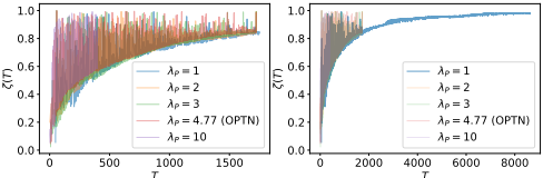
Figure 1: Kidney Exchanges Approaching Steady-State. On the left, we plot the steady-state parameter ζ(T) for simulated kidney exchanges of varying size for 10,000 days. On the right, we extend the plot for the smallest exchange (for computational reasons) to 50,000 days.
at iteration T as
For simplicity, we define AT := ∑Tt=1 |A(t)| and DT := ∑Tt=1 |D(t)|. Note that ζ(T) ∈ [0, 1]. A kidney exchange in steady-state should have ζ(T) ≈ 1, as the total number of departures should approach the total number of arrivals. Although extremely intractable to study analytically, Figure 1 shows that the stochastic function ζ(T) follows a highly well-behaved lower-bound, no matter the size of exchange. Interestingly, as shown in the right plot of Figure 1, ζ(T) suddenly appears to become much-less noisy after it passes the inflection point of this lower bound.
5.2 Relating Distributional Shift to the Steady-State Parameter
We now show how the distributional shift can be bounded in terms of ζ(T). Let RT = {u1, . . . uDT } be the set of vertices in the match record. We further have that RT ⊆ ⋃Tt=1 A(t) := {v1, . . . , vAT }. To make the analysis tractable, we assume that the feature space F = Rd is continuous, and that the distribution over the features of any arrival vi ∼ fP = N (µ, Σ) are jointly Gaussian with mean µ and full-rank covariance Σ. We measure the distributional shift by considering shifted directions - directions in which the training data differs statistically from the test distribution. Formally, we say that a unit vector z ∈ Rd is δ-shifted if
Here Φ refers to the CDF of a standard normal variable. This definition basically requires that the Kolmogorov distance between the empirical CDF of the projected data from the match record and the true CDF of the projected arrivals exceeds δ. We say that RT is (γ, δ)-shifted if there is a set of δ-shifted directions that have uniform measure γ (or in other words, Prz∼N(0,I) [ z ∥z∥2 is δ-shifted] > γ). We show that when ζ(T) ≈ 1, RT is not (γ, δ)-shifted with high probability - that is, if the kidney exchange is at steady-state, the match record cannot be shifted in too many directions. As RT ⊆ ⋃Tt=1 A(t) is a (perhaps even adversarially/arbitrarily chosen) subset of the arrivals, its entries are not distributed as N (µ,Σ). We can, however, upper bound the probability that RT is (γ, δ)-shifted by taking the union bound over all fixed coalitions of size DT in ⋃Tt=1 A(t). If ζ(T) is large, then there cannot be too many of these coalitions. This simplification is useful, as the features of any fixed coalition of vertices in ⋃Tt=1 A(t) are normally distributed as N (µ, Σ).
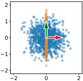
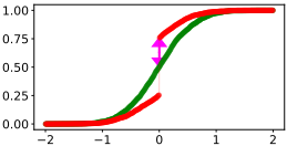
Using standard tools from empirical process theory (namely the DKWM inequality. restated as Lemma D.1), we show using a probabilistic approach that RT is a (γ, δ)- shifted with low probability:
Theorem 5.1. Let RT = ⋃Tt=1 D(t) denote the match record at time T, and let any vertex vi ∈ ⋃Tt=1 A(t) have features that are normally distributed as N (µ,Σ) where Σ is full rank. Then,
The full proof of Theorem 5.1 can be found in Appendix D. Figure 3 shows how our bounds vary with ζ(T), AT , and d. If the feature space is lower dimensional (e.g., d ≈ 10), we find that our bound produces trivial results when ζ(T ) ⪅ 0.8. Immediately after this threshold, however, the probability that the match record is shifted becomes astronomically small. Interestingly, as the dimensionality d of the feature space increases, the well-known "curse of dimensionality" in fact behaves as a blessing. High dimensional space contains many directions, and it is difficult for an adversary to shift the distribution in a constant fraction of these at once. This is reflected in our bound, as we see that the probability decreases exponentially in d. We visualize this phenomenon in Figure 3 - even small exchanges (corresponding to a small value for AT ) that are not in steady-state (i.e., ζ(T) ≈ 0) remain unshifted when the dimension d exceeds 30.
In practice, many fielded exchanges have been observed to be at or near steady-state [Bir´o et al., 2019], and matching policies tend to make use of at least 20-30 features [OPTN, 2021]. However, as demonstrated in Section 7, only 10-20
are highly relevant for prediction. Thus, we obtain some benefits from the dimensionality, but perhaps not enough to eliminate the distributional shift in kidney exchanges far from steady-state.
6 Experiments
We now evaluate our random forest approach on simulated match data. For varying arrival rates λP corresponding to kidney exchanges of different sizes, we use the batch simulator described in Section 4.2 to generate simulated match records RT . We generate test data for each of these pools by running the trajectory simulator with S = 300 samples and τ = 500 trajectories. Trajectory simulation is very computationally intensive, taking about a week to terminate on an HPC cluster. We set T = 259, which corresponds to D = 1500 days (or roughly 4 years), to prevent pool sizes for the larger exchanges we tested from becoming too large. We also tested our two smallest exchanges setting D = 4000 days (or roughly 11 years), and our smallest exchange setting D = 50000 days (or roughly 136 years) to understand the performance of our approach on older kidney exchanges. The OPTN exchange is now 11 years old, so our experiments for D = 4000 (in addition to those for D = 1500) do correspond to benchmarks for realistic exchanges. With the exception of the D = 50000 experiment, we re-run all experiments in a federated learning setting where 5 exchanges of the same age aggregate their match records together for prediction. When we aggregate the match records of similar exchanges together, we increase the size of the training dataset while keeping the steady state parameter ζ (and thus the distributional shift) roughly the same. Thus, these experiments allow us to understand whether poor performance is due to insufficient data or distributional shift.
As described in Section 3, we use a random forest classifier to predict the outcome O(v), and we use quantile regression forests to produce 95% prediction intervals for the waiting time W(v) and quality Q(v) conditioned on a match. Letting v∗ 1 , . . . , v∗S denote the S samples drawn by the trajectory simulator, we evaluate our classifier by computing the mean absolute error MAE ( ̂O) := 1S ∑Si=1 ∣∣∣ ̂O(v∗ i ) - Pr [O(v∗ i ) = 1]∣∣∣. We evaluate the prediction intervals ̂ W95 and ̂Q95 using the mean intersection over union (IOU), which computes the length of the intersection of the intervals divided by the length of the union of the intervals IOU(̂ W95) = 1S ∑Si=1 |̂ W95(v∗ i )∩W95(v∗ i )| |̂ W95(v∗ i )∪W95(v∗ i )| . We estimate the true parameters Pr [O(v∗ i ) = 1], W95(v∗ i ), and Q95(v∗ i ) from the τ sampled trajectories.
Table 3 shows our experimental results. We consider MAE scores less than 0.2 and IOU scores greater than 0.5 as good performance. The classifier performance MAE( ̂O) seems to primarily be determined by the dataset size. This is especially evident in the federated setting, where aggregating multiple match records together always improved performance by as much as 7.6%. Performance for waiting time prediction, on the other hand, appears to be highly dependent on the steadystate parameter. The IOU scores for waiting time can roughly be sorted by ζ, and do not necessarily increase in the federated setting, indicating that distributional shift is likely affecting the result. Predicting the organ quality appears to be an easy task - every experiment produced good performance, well exceeding our benchmark IOU of 0.5. This is especially impressive, as the smallest exchange we tested had a match record with only 56 entries. Federated learning improved scores in all cases but one.

| Arrival Rate | D | Federated | |RT | | ζ | MAE ( ̂O) | IOU (̂ W95) | IOU ( ̂Q95) |
|---|---|---|---|---|---|---|---|
| λP = 1 | 1500 | No | 56 | 0.397 | 0.258 | 0.451 | 0.747 |
| λP = 1 | 4000 | No | 246 | 0.953 | 0.191 | 0.644 | 0.761 |
| λP = 1 | 50000 | No | 4888 | 0.984 | 0.130 | 0.653 | 0.632 |
| λP = 2 | 1500 | No | 157 | 0.477 | 0.221 | 0.336 | 0.815 |
| λP = 2 | 4000 | No | 752 | 0.882 | 0.212 | 0.620 | 0.809 |
| λP = 3 | 1500 | No | 285 | 0.523 | 0.184 | 0.386 | 0.798 |
| λP ≈ 4.77 (OPTN) | 1500 | No | 593 | 0.509 | 0.164 | 0.503 | 0.812 |
| λP = 1 | 1500 | Yes | 268 | 0.457 | 0.246* | 0.232 | 0.816* |
| λP = 1 | 4000 | Yes | 1224 | 0.891 | 0.148* | 0.590 | 0.800* |
| λP = 2 | 1500 | Yes | 807 | 0.550 | 0.145* | 0.373* | 0.816* |
| λP = 2 | 4000 | Yes | 3773 | 0.872 | 0.119* | 0.775* | 0.820* |
| λP = 3 | 1500 | Yes | 1434 | 0.488 | 0.115* | 0.421* | 0.815* |
| λP ≈ 4.77 (OPTN) | 1500 | Yes | 2652 | 0.537 | 0.103* | 0.449 | 0.812 |
Overall, our experiments demonstrate that kidney exchanges of any size that are roughly 4000 days or older may use existing match records to make clinically promising estimates for O(v), W(v), and Q(v). Young exchanges that are relatively large may not be able to able to produce good estimates for waiting time, but can still estimate O(v) and Q(v) reliably well. Young exchanges that are also small likely cannot estimate the match outcome O(v) or the waiting time W(v), but can still provide patients with good estimates for the organ quality Q(v). Although highly exploratory in nature, our experiments also suggest that federated learning can improve performance - especially when predicting O(v).
7 DiagnosingMechanismBehavior with SHAP Analysis
In Sections 5 and 6, we demonstrated how, at least for relatively older exchanges, it is possible to train random forest models to produce good estimates for the match outcomes O(v), W(v), and Q(v). These models may serve as decisionsupport tools to help patients and healthcare workers with medical and insurance decisions. We show how the utility of these models extends beyond this domain - using Shapley additive explanations (SHAP) to compute feature importances [Lundberg and Lee, 2017; Lundberg et al., 2018], in addition to t-Distributed Stochastic Neighbor Embeddings (tSNE) [Van der Maaten and Hinton, 2008] for visualization, we can use these models to help kidney exchange policymakers understand how the underlying matching mechanism treats different groups of patients. In Appendix 7, we give background on these techniques, an in-depth explanation of our approach, and a demonstration of its use (and our findings). Although we perform this analysis using data from our simulated OPTN exchange, we emphasize that these techniques may be readily applied to any fielded exchange as our approach only makes use of data from existing match records.
8 Discussion
We proposed and validated a random forest approach to forecast patient outcomes in kidney exchange. We provide strong theoretical and experimental evidence in a state-of-the-art kidney exchange simulation framework that the match outcome O(v), the waiting time W(v), and the organ quality Q(v) can be reliably estimated in older fielded exchanges of any size. Further, W(v) can be estimated well in larger young exchanges, and Q(v) can be estimated well even in smaller young exchanges. As our approach exclusively makes use of existing match records, it may be readily deployed as a decision-support tool in exchanges across the world. Our tool doubles as a principled method for detecting bias and policy miscalibration, and may be used to inform kidney exchange policy; we view this as one step towards increased agency and transparency in kidney exchange.
Acknowledgements
Srinivasan was supported in part by NSF Award CCF1749864, and by research awards from Adobe, Inc., Amazon, Inc., and Google Inc. Dickerson was supported in part by NSF CAREER Award 184623.
@inproceedings{ijcai2022p701,
  title     = {Forecasting Patient Outcomes in Kidney Exchange},
  author    = {Durvasula, Naveen and Srinivasan, Aravind and Dickerson, John},
  booktitle = {Proceedings of the Thirty-First International Joint Conference on
               Artificial Intelligence, {IJCAI-22}},
  publisher = {International Joint Conferences on Artificial Intelligence Organization},
  editor    = {Luc De Raedt},
  pages     = {5052--5058},
  year      = {2022},
  month     = {7},
  note      = {AI for Good},
  doi       = {10.24963/ijcai.2022/701},
  url       = {https://doi.org/10.24963/ijcai.2022/701},
}
TY - CPAPER TI - Forecasting Patient Outcomes in Kidney Exchange AU - Durvasula, Naveen AU - Srinivasan, Aravind AU - Dickerson, John T2 - Proceedings of the Thirty-First International Joint Conference on Artificial Intelligence, IJCAI-22 PB - International Joint Conferences on Artificial Intelligence Organization PY - 2022 SP - 5052 EP - 5058 DO - 10.24963/ijcai.2022/701 UR - https://doi.org/10.24963/ijcai.2022/701 ER -Copied
Machine-readable versions of this paper, for tools and AI agents:





