
Learning Constraint Networks over Unknown Constraint Languages
Proceedings of the Thirty-Second International Joint Conference on Artificial Intelligence. Main Track. Pages 1876-1883.
https://doi.org/10.24963/ijcai.2023/208
Keywords
- Constraint Satisfaction and Optimization: CSO: Constraint programming
- Constraint Satisfaction and Optimization: CSO: Constraint learning and acquisition
Abstract
Constraint acquisition is the task of learning a constraint network from examples of solutions and non-solutions. Existing constraint acquisition systems typically require advance knowledge of the target network's constraint language, which significantly narrows their scope of applicability. In this paper we propose a constraint acquisition method that computes a suitable constraint language as part of the learning process, eliminating the need for any advance knowledge. We report preliminary experiments on various acquisition benchmarks.
- [Beldiceanu and Simonis, 2012] Nicolas Beldiceanu and Helmut Simonis. A model seeker: Extracting global constraint models from positive examples. In Michela Milano, editor, Principles and Practice of Constraint Programming -18th International Conference, CP 2012, Québec City, QC, Canada, October 8-12, 2012. Proceed- ings, volume 7514 of Lecture Notes in Computer Science, pages 141-157. Springer, 2012.
- [Bessiere et al., 2005] Christian Bessiere, Remi Coletta, Frédéric Koriche, and Barry O'Sullivan. A sat-based ver- sion space algorithm for acquiring constraint satisfaction problems. In João Gama, Rui Camacho, Pavel Brazdil, Alípio Jorge, and Luís Torgo, editors, Machine Learn- ing: ECML 2005, 16th European Conference on Machine Learning, Porto, Portugal, October 3-7, 2005, Proceed- ings, volume 3720 of Lecture Notes in Computer Science, pages 23-34. Springer, 2005.
- [Bessiere et al., 2009] Christian Bessiere, Emmanuel He- brard, Brahim Hnich, Zeynep Kiziltan, and Toby Walsh. Range and roots: Two common patterns for specifying and propagating counting and occurrence constraints. Artif. In- tell., 173(11):1054-1078, 2009.
- [Bessiere et al., 2017] Christian Bessiere, Frédéric Koriche, Nadjib Lazaar, and Barry O'Sullivan. Constraint acquisi- tion. Artif. Intell., 244:315-342, 2017.
- [Kumar et al., 2019] Mohit Kumar, Stefano Teso, and Luc De Raedt. Acquiring integer programs from data. In Sarit Kraus, editor, Proceedings of the Twenty-Eighth International Joint Conference on Artificial Intelligence, IJCAI 2019, Macao, China, August 10-16, 2019, pages 1130-1136. ijcai.org, 2019. IJCAI
- [Kumar et al., 2022] Mohit Kumar, Samuel Kolb, and Tias Guns. Learning constraint programming models from data using generate-and-aggregate. In Christine Solnon, editor, 28th International Conference on Principles and Practice of Constraint Programming, CP 2022, July 31 to August 8, 2022, Haifa, Israel, volume 235 of LIPIcs, pages 29:1- 29:16. Schloss Dagstuhl -Leibniz-Zentrum für Informatik, 2022.
- [Pawlak and Krawiec, 2017] Tomasz P. Pawlak and Krzysztof Krawiec. Automatic synthesis of constraints from examples using mixed integer linear programming. Eur. J. Oper. Res., 261(3):1141-1157, 2017.
- [Piotrów, 2020] Marek Piotrów. Uwrmaxsat: Efficient solver for maxsat and pseudo-boolean problems. In 32nd IEEE International Conference on Tools with Artificial Intelli- gence, ICTAI 2020, Baltimore, MD, USA, November 9-11, 2020, pages 132-136. IEEE, 2020.
- [Prestwich et al., 2021] Steven D. Prestwich, Eugene C. Freuder, Barry O'Sullivan, and David Browne. Classifier- based constraint acquisition. Ann. Math. Artif. Intell., 89(7):655-674, 2021.
References were extracted automatically from the PDF and may contain errors.
Full text extracted automatically from the PDF; figures, tables and equations may differ. The PDF is the version of record.
1 Introduction
Constraint programming (CP) is a powerful technology for solving combinatorial problems. It has gained significant attention in the last decades. Its ability to efficiently solve complex problems has made it a popular choice for a variety of real-world applications. However, one bottleneck in the use of CP is the process of expressing the problem with constraints, which often requires advanced knowledge in both CP and the problem to model.
Constraint acquisition addresses this issue by automatically generating a model from examples of past solutions or non-solutions, or by asking queries of the user. In this paper, we are interested in passive learning approaches, that is, those in which the user provides a set of solutions and non-solutions of a target model.
Given a set of examples of solutions and non-solutions and a set of candidate constraints, CONACQ.1 computes a SAT formula representing all the constraint models expressed with constraints from the candidate set and consistent with the examples [Bessiere et al., 2005; Bessiere et al., 2017]. Given a set of examples, MODELSEEKER proposes a set of constraints taken from the global constraints catalog that are consistent with the given examples [Beldiceanu and Simonis, 2012]. As proposing all possible constraints to the user would be far too heavy, MODELSEEKER is limited to constraints involving variables from a common topology, such as rows or columns in a matrix. BAYESACQ follows a statistical approach [Prestwich et al., 2021]. BAYESACQ takes as inputs a set of examples and a set of candidate constraints. For each candidate constraint, BAYESACQ computes a score based on the ratio of the number of negative examples the constraint violates to the number of positive examples it violates. These ratios are used to return the most probable set of constraints. The method presented in [Pawlak and Krawiec, 2017] expresses the constraint acquisition problem as a mixed integer linear programming problem whose solutions are sets of constraints correctly classifying all examples. The constraints can be taken from the sets of linear, quadratic or trigonometric constraints, depending on the problem to model.
All the constraint acquisition approaches cited above require knowledge of the constraint language that is used to generate the set of candidate constraints. This narrows the scope of applicability of these approaches because a nonexpert user might not be able to provide a constraint language that suits his problem. The objective of this paper is to present a general approach where constraint acquisition only requires the user to provide a set of examples of solutions and nonsolutions of the target constraint network. No set of candidate constraints is required. We first define the decision version of the constraint acquisition problem over unknown constraint language when the maximum number k of relations in the unknown language and the maximum arity r of its relations are given. We prove that the problem is NP-complete, even when k = r = 1. Given a number k of relations and an arity r, we encode the problem of finding a constraint network over unknown language as a partial maximum satisfiability problem. We then propose a method to solve the problem of finding a constraint network over unknown language when k and r are not given. We just need to assume a preference order on the pairs (k, r). We finally validate our method by analyzing its behavior on a set of benchmark problems.
There already exist a couple of approaches that could be considered as very close to ours because they do not explicitly require the set of candidate constraints to be given as input to the acquisition problem. ARNOLD learns integer programs from examples of feasible solutions by generating potential constraints that only include sums, products, and comparisons among of terms [Kumar et al., 2019]. The generation of constraints follows a general-to-specific order and collects those that are satisfied by the example solutions in order to produce an integer program model. COUNT-CP also learns a network of constraints from examples of solutions [Kumar et al., 2022]. COUNT-CP uses a grammar and a generateand-aggregate approach to determine the constraints on this grammar from the examples. Though not explicitly given as input, the generated constraints must belong to the language of the given grammar, which is able to express a large bunch of "counting" constraints (see [Bessiere et al., 2009]), but is not able to express any kind of constraints.
The rest of this paper is organized as follows. In Section 2, we provide background on constraint acquisition. In Section 3, we present the formalization of constraint acquisition problem over unknown constraint languages and we prove that it is NP-complete. In Section 4, we describe our method. In Section 5, we study the effectiveness of our method through several experiments. Finally, in Section 6, we conclude with a summary of our contribution and we discuss directions for future work.
2 Background
2.1 Constraint Programming
Constraint programming consists in expressing a problem as a constraint network and finding solutions, that is, assignments of values to all the variables so that no constraint is violated. Given a domain D, a constraint is a pair ⟨R, S⟩, where R is a relation of arity r over D (that is, R is a subset of Dr ) and S is a sequence of r variables (called the scope of the constraint). A vocabulary is a pair ⟨X, D⟩, where X is a finite set of variables and D is a finite domain. An assignment A : X → D satisfies a constraint ⟨R, S⟩ if A[S] ∈ R; otherwise, the assignment violates the constraint.
Definition 1 (Constraint network). A constraint network is a tuple N = ⟨X,D,C⟩, where ⟨X,D⟩ is a vocabulary and C is a set of constraints on subsets of X. An assignment A : X → D satisfies N iff A satisfies all constraints in C.
A constraint language Γ is a set of relations over a finite domain. The arity of Γ is the maximum arity over all relations of Γ. A constraint network N is over a constraint language Γ if the relation R of each constraint of N is such that R ∈ Γ.
2.2 Constraint Acquisition
Given a vocabulary ⟨X,D⟩, an example on this vocabulary is a pair e = ⟨ϕ(e), b(e)⟩, where ϕ(e) is an assignment, and b(e) is a Boolean. We say that e is a positive example if b(e) is true; otherwise e is a negative example. We say that a constraint network N accepts (resp. rejects) an example e iff ϕ(e) satisfies (resp. does not satisfy) N. A constraint network N is consistent with a positive (resp. negative) example e if and only if N accepts (resp. rejects) e
A training set E is a set of examples over a given vocabulary. A constraint network N is consistent with a training set E if and only if N is consistent with every example in E. Given a training set E, E+ (resp. E-) denotes the subset of all positive (resp. negative) examples of E.
2.3 Boolean Satisfiability
As our method will use a WEIGHTED PARTIAL MAX-SAT solver, we introduce some basics about Boolean satisfiability. A literal is a Boolean variable or its negation. A clause is a disjunction of literals. The Boolean satisfiability problem (SAT) on a set of clauses CL asks whether it is possible to assign values to the variables of CL such that all clauses are satisfied, i.e. CL evaluates to True. If µ is a truth assignment of Boolean variables and l is a literal, we will slightly abuse notation and write µ(l) to denote the truth value of l under µ. The partial maximum satisfiability problem, PARTIAL MAX-SAT, is a variant of SAT in which the goal is to find an assignment such that all clauses in a first set called hard clauses are satisfied, and the number of satisfied clauses in another set of clauses called soft clauses is maximized. In the WEIGHTED PARTIAL MAX-SAT problem, each soft clause has a weight and we maximize the sum of the weights of satisfied soft clauses.
3 Language Acquisition
In this paper, we consider the constraint acquisition problem without any language of constraints or set of candidate constraints given as input data. Rather than working with a fixed constraint language, we compute a constraint language Γ alongside a constraint network over Γ that is consistent with the training set.
An important difficulty with this approach is that there may exist a large number of constraint languages that are consistent with a given training set. Some of these languages are clearly unsatisfactory from a practical point of view; for example, every training set over n variables is trivially consistent with a constraint network over a constraint language of arity n and size 1. This constraint network has a single constraint covering all variables. Its satisfying assignments are exactly the positive examples in the training set.
Our intuition is that the best constraint language is the simplest. Because "simplicity" is difficult to define formally, we instead consider (as a first, rough approximation) that the best language is the smallest in terms of its maximum arity and number of relations. This leads us to the following definition for the constraint acquisition problemwithout language.
Definition 2 (LANGUAGE-FREE ACQ). Given a training set E and two natural numbers k, r, the problem LANGUAGEFREE ACQ asks whether there exists a constraint network over a language of size at most k and arity at most r consistent with E.
In practice we will solve an optimization and search variant of this problem, in which we attempt to find a constraint network with minimum (k, r) that is consistent with E. The problem is multi-objective (both the language arity and size must be minimized), so multiple strategies are possible: for example, one could define a real-valued cost function f(k, r) to be minimized or compute a Pareto front. The next theorem states that LANGUAGE-FREE ACQ is NP-complete even when (k, r) = (1, 1), so solving the optimization/search variant is likely to be difficult regardless of the chosen strategy.
Theorem 1. LANGUAGE-FREE ACQ is NP-complete even when k = r = 1.
Proof. We first prove membership in NP. Suppose that there exists a constraint network N = (X,D,C) over a language Γ = (R1, . . . , Rk) of arity r and size k that is consistent with E. We can further assume that each constraint rejects at least one negative example that is accepted by all other constraints, in which case N has at most |E| constraints. We specify each relation Rj ∈ Γ succinctly by listing only the tuples t ∈ Rj such that there exists a constraint c = (Rj , S) and an example e ∈ E such that ϕ(e)[S] = t; the number of such tuples is at most |C| · |E| ≤ |E|2 . This succinct representation of N has polynomial size (even when r, k are part of the input) and can be checked for consistency with E in polynomial time, so LANGUAGE-FREE ACQ ∈ NP.
In order to prove NP-hardness, we reduce SAT to LANGUAGE-FREE ACQ. Let CL = {Z1,Z2, ...,Zm} be a set of m clauses over a set V = {v1, v2, ..., vn} of n Boolean variables. We define a training set E over a vocabulary ⟨X,D⟩ with X = {xv | v ∈ V } ∪ {x¬v | v ∈ V } and D = {v | v ∈ V } ∪ {¬v | v ∈ V } ∪ {⋆} such that:
- e+⋆ ∈ E+ such that ∀x ∈ X, ϕ(e+⋆ )[x] = ⋆
- ∀v ∈ V, e+v ∈ E+ such that:
- ∀v ∈ V, e-v ∈ E- such that:
We claim that there exists a constraint network N = ⟨X, D, C⟩ over a language {R} of size 1 and arity 1 which is consistent with E if and only if CL is satisfiable.
Let us assume that there exists such a network N consistent with E. We show that this implies that CL is satisfiable. N must accept e+⋆ , so ⋆ ∈ R. For each v ∈ V , N must reject e-v . Hence, we have either v /∈ R and ⟨R, {xv}⟩ ∈ C, or ¬v /∈ R and ⟨R, {x¬v}⟩ ∈ C. We cannot have both v and ¬v forbidden by R because e+v must be accepted by N. We thus have exactly one among v and ¬v forbidden by R, and we can define the assignment µ : V → {False, True} such that for each v ∈ V we have µ(v) = True ⇔ v /∈ R and µ(v) = False ⇔ ¬v /∈ R. We also know that for all Z ∈ CL, N has to reject e-Z . Now, ϕ(e-Z )[x] = ⋆ for all x except those literals composing Z. As a result, there is at least one literal l in Z such that l /∈ R, and then µ(l) = True. We conclude that µ satisfies CL.
Let us now assume that there exists an assignment µ that satisfies CL. We show that this implies that there exists a network N = (X,D,C) over a language {R} of size 1 and arity 1 which is consistent with E. We define the relation R = D\{l | µ(l) = True} and C = {⟨R, ⟨xv⟩⟩ | ∀v ∈ V, µ(v) = True} ∪ {⟨R, ⟨x¬v⟩⟩ | ∀v ∈ V, µ(v) = False}. N accepts e+⋆ because ⋆ ∈ R. For all v ∈ V , either ⟨R, {xv}⟩ ∈ C with ¬v ∈ R and v /∈ R, or ⟨R, {x¬v}⟩ ∈ C with v ∈ R and ¬v /∈ R, but not both. Hence, N accepts e+v and rejects e-v . As µ satisfies CL, for each Z ∈ CL, there exists l ∈ Z such that µ(l) = True. Thus, ⟨R, {xl}⟩ ∈ C with l /∈ R and N rejects e-Z . We conclude that the network N constructed above, which is over a language {R} of size 1 and arity 1, is consistent with E.
Both N and E are computable in polynomial time from CL.
4 Solving the LANGUAGE-FREE ACQ Problem
In this section we present our method for constraint acquisition, which is based on repeatedly solving instances of the LANGUAGE-FREE ACQ problem.
4.1 Method Overview
Given a training set E, our goal is to compute a constraint network consistent with E with minimum (k, r). As noted in Section 3, multiple strategies are possible. The most direct approach would be to output a constraint network with minimum k + r. We believe that increasing the arity should incur a greater penalty than increasing the number of relations, so we will minimize k + r2 instead. We break ties by giving preference to lower arity (for example, six relations of arity two are preferred over one relation of arity three).
It may be the case that multiple constraint networks have the same arity and number of distinct relations. In that case, we output a network with the largest number of constraints. Our intuition behind this decision is that for sufficiently large training sets, the fact that few relations can be applied to many scopes without rejecting any positive example is unlikely to be observed by chance. For the same reason, if multiple constraint networks have the same (k, r) and number of constraints, we output one whose constraints are the tightest, i.e. whose relations contain the fewest tuples on aggregate.
For fixed (k, r), we compute the desired constraint network (or prove that none exists) using a WEIGHTED PARTIAL MAX-SAT model, which we describe in the next sub-section. Since our model is particularly efficient for small values of (k, r), we perform bottom-up minimization, constructing and solving a model for each (k, r) by increasing order of k + r2 . We then output the first constraint network found.
4.2 The Model
Suppose that (k, r) is fixed. Our goal is to compute a constraint network N = ⟨X,D,C⟩ over a language of size k and arity r that is consistent with E, whose number of constraints is maximum, and with the tightest constraints possible. We model this optimization problem as an instance of WEIGHTED PARTIAL MAX-SAT. In the following, RT(E) will denote the set of all pairs (t, v) such that t ∈ Dr , v ∈ Xr , and there exists an example e in E such that t = ϕ(e)[v].
For each relation Ru of the target language {R1, . . . ,Rk}, we have three kinds of Boolean variables in the WEIGHTED PARTIAL MAX-SAT model:
- For all t in Dr , ru t is true iff t /∈ Ru;
- For all v in Xr , suv is true iff ⟨Ru, v⟩ ∈ C;
- For all (t, v) in Dr ×Xr , cu(t,v) ≡ ru t ∧ suv .
First, for each (u, t, v) ∈ {1, ..., k} ×Dr ×Xr , we ensure that cu(t,v) ≡ ru t ∧ suv with the following hard clauses:
Second, we make sure that all positive examples are accepted by the corresponding constraint network with the following set of hard clauses:
Similarly, we make sure that all negative examples are rejected:
Finally, in order to maximize the number of constraints in the network and, in a second time, minimize the number of tuples in the relations, we add a soft clause (suv ) with weight 1 for each u ∈ {1, . . . , k} and v ∈ Xr , and a soft clause (ru t ) with weight ϵ < 1/(k · |Dr |) for each u ∈ {1, . . . , k} and t ∈ Dr . This completes the description of the model.
The size of this WEIGHTED PARTIAL MAX-SAT model is defined by its number of clauses and their sizes. The number of -constant-size- clauses of type (1) and (2) is O(|D|r ·|X|r · k). There are |E-| clauses of type (3), each of size bounded above by |D|r · |X|r · k. Finally, the number of -constantsize- soft clauses (suv ) and (ru t ) is bounded above by (|X|r + |D|r ) · k . This gives a total size of our model in O(|E-| · |D|r · |X|r · k).
Observe that the exponential dependency on the maximum arity r is not a necessary feature of all models for this problem because LANGUAGE-FREE ACQUISITION is in NP (even when r is part of the input). However, this model has the advantage of being flexible (it is easy, for example, to maximize the number of constraints in the learned constraint network) and very efficient for small values of r. In addition, this upper bound is quite loose as not all variables/clauses need to be generated. For any u, t, v such that (t, v) /∈ RT(E-), we do not need to generate the variable cu(t,v) and the corresponding clauses of type (1) because it will never appear in the clauses of type (2) or (3). The same is true for all u, t, v such that (t, v) ∈ RT(E+). These refinements are particularly effective when the number of examples is small.
Finally, we note that the model contains some symmetries. For example, its solution set is invariant under permutation of the relational indices u ∈ {1, . . . , k} and permutation of the entries of (t, v) for a fixed u. These symmetries can easily be broken using standard techniques. It was unnecessary for our experiments as k, r were always fairly small.
5 Experimental Results
In this section, we evaluate our method experimentally on several benchmark problems. For each benchmark, we will investigate how the number of examples affects the accuracy of the learned constraint network, the similarity of the learned constraint network with the target (Are they over the same constraint language? Are they logically equivalent? Are they exactly identical?), and the observed runtime. We will then dive deeper into the details for an archetypal benchmark of constraint acquisition (the sudoku), examining in particular how the fraction |E+|/|E| of positive examples in the training set affects the learning process.
We have implemented the strategy described in Section 4.1 in the Python programming language. Our program takes as input a training set, generates the corresponding WEIGHTED PARTIAL MAX-SAT instances and calls an external solver given by the user as a parameter. We chose to use the UWRMAXSAT solver [Piotr´ow, 2020]. All experiments 1 are run on one core of an Intel Xeon E5-2680 v4 2.4GHz processor with 8GB of memory.
5.1 Benchmark Problems
Sudoku
The Sudoku is a logic puzzle with a 9 × 9 grid that must be filled with the digits 1 to 9 in such a way that all the rows, all the columns and 9 non-overlapping 3 × 3 squares contain all the digits from 1 to 9. For this problem, the target constraint network has 81 variables x1, . . . , x81, domains of size 9, and a binary constraint xi ̸= xj for all i, j in the same row, column or square. Positive examples are generated by computing solutions of the target constraint network with a constraint solver using a randomized domain value strategy. Non-solutions are generated by altering one value in a solution randomly.
Jigsaw Sudoku
The Jigsaw Sudoku is a variant of the Sudoku in which the partition in 3 × 3 squares is replaced by a partition into nonoverlapping, irregular shapes of size 9 called jigsaw shapes. The irregularity of the jigsaw shapes makes Jigsaw Sudoku particularly difficult (or even impossible) to learn for methods that rely heavily on predefined constraint topologies, such as MODELSEEKER. For this problem, the target constraint network has 81 variables x1, . . . , x81, domains of size 9, and a binary constraint xi ̸= xj for all i, j in the same row, column or jigsaw shape. Examples are generated in the same way as for Sudoku.
We have observed significant variance in experimental results for different types of jigsaw shapes. To reflect this, we have divided these benchmarks into three sub-families (#1, #2 and #3) corresponding to three different layouts.
Schur's Lemma
The problem is to put n balls labelled 1, · · · , n into 3 boxes so that for any triple of balls (x, y, z) with x + y = z, not all are in the same box. For this problem, the target constraint network has n variables x1, . . . , xn, domains of size 3, and a ternary constraint NotAllEqual(xi, xj, xk) for all i, j, k such that i + j = k. We ran the experiment with n = 9 which is the parameter with the highest number of solutions (546). Positive examples are generated by computing solutions of the target constraint network with a constraint solver using a randomized domain value strategy. Non-solutions are generated by altering one value in a solution randomly.
1 Code and data required for conducting the experiments are available at https://gite.lirmm.fr/coconut/language-free-acq
Subgraph Isomorphism
Given two graphs G and H, subgraph isomorphism is the problem of determining whether G contains a subgraph that is isomorphic to H. For this problem, the target constraint network has |H| variables x1, . . . , xn and domains of size |G|. A binary constraint xi ̸= xj for all i, j ensures that the mapping between the vertices of H and G is a one-to-one function and another binary constraint ensures that for any edge (a, b) in H, (xa, xb) is an edge of G. We ran the experiment with H a cycle of size 5 and a new random graph G for each run having 20 vertices and 100 edges. Positive examples are generated by computing solutions of the target constraint network with a constraint solver using a randomized domain value strategy. Non-solutions are paths and closed walks of G computed using a randomized domain value strategy.
N-Queens
The N-Queens problem is the problem of placing N queens on a N ×N chessboard such that no two queens can attack each other. For this problem, we use the standard representation in which there is a variable per column. The target constraint network has N variables x1, . . . , xN, where xi represents the row in which the queen on the ith column is positioned. All domains are {1, . . . ,N}. There are binary constraints xi ̸= xj and |xi -xj| ̸= |i-j| for all i, j. This gives us a language of size N corresponding to all possible values of |i - j|. The constraint language is binary and has size N. We ran the experiment with N = 8, for which the problem has 92 solutions. We generate positive examples by computing a random solution, and negative examples by randomly permuting the values or altering one value in a solution.
Golomb Ruler
The Golomb Ruler problem is the problem of finding a set of marks on a ruler such that the difference between any two marks is unique. The target constraint network has n variables, each representing the position of a mark on the ruler, domains of fixed size {0...m}, and a quaternary constraint |xi - xj| ̸= |xk - xl| for all i, j, k, l. For the experiment, we choose to use n = 10 and m = 60. Positive examples are generated by computing a random solution of the target constraint network with the symmetry breaking constraint xi < xj for all i < j and then randomly permuting the values of this solution. Non-solutions are generated by altering one value in a solution randomly.
5.2 Network and Language Acquisition
In this first experiment, we evaluate the overall performance of our method on the acquisition of our benchmark problems. We first present the experimental protocol and then discuss important points in the results.
Protocol
We conduct a series of experiments with different numbers of examples in the training sets. For each benchmark problem and number |E| of examples, we run our acquisition method 5 times with a new randomly sampled training set for each run. Training sets contain positive and negative examples in the same proportion. The timeout is set to 12 hours. The performance of the model is measured in terms of the average accuracy over the five runs, which is computed on a new set of 2000 examples generated independently. We also record the optimal (k, r) values found, the number of times the learned language is the target language (out of the 5 runs), the number of times the learned network is equivalent to the target network (i.e. they have exactly the same solutions) and the number of times the learned network is precisely the target network (i.e. with exactly the same constraints). We finally record the average runtime of the acquisition process, including the time required to prove that there does not exist any network consistent with E for values of (k, r) smaller than the (optimal) one returned.
Results
We provide a summary of the results in Table 1. The target network for the Sudoku problem is consistently learned (that is, learned for all 5 runs) with 200 examples in the training set, and even as few as 100 examples in 2 runs out of 5. The Jigsaw Sudoku required significantly more examples before reaching 100% accuracy, from 600 to 1400 depending on the jigsaw shapes. For this problem, the target constraint network is never learned no matter the size of the training set. Equivalent networks are learned instead, which we observed to correspond to the target network with additional redundant constraints. (For the classical Sudoku, all possible redundant inequality constraints are already included in the target network. This is not true for all jigsaw shapes.) For Schur's Lemma, with only 50 examples the target constraint language is consistently learned and the accuracy is above 85%. This is particularly interesting because this language has arity 3, so this means that all constraint languages with at most 6 binary relations can be ruled out with very few examples. Learning the target network consistently requires up to 800 examples, even if 2 runs out of 5 succeeded with only 200. Subgraph isomorphism is the first problem for which the target language contains two relations. With 100 examples, the learned networks are over a language with a single relation and the accuracy is below 60%. 100% accuracy and equivalent networks are reached with 800 examples, although the target network and language can never be learned. This is because it is theoretically not possible to distinguish the graph G (whose edges correspond to the tuples of one relation in the target language) from another graph G′ with identical 5cycles using only examples. For the 8-Queens problem, the experiment is limited to at most 184 examples because the problem has only 92 solutions and we need 50% of positive examples in the training set. We observe that even training sets with 184 examples are not sufficient to reach 100% accuracy or learn the target constraint language (which is of size 8). Instead, our method outputs constraint networks over languages of size only 3 that achieve 99% accuracy. The Golomb Ruler is particularly challenging because the target language has arity 4. Runtimes are extremely high, with the 12-hour timeout being reached for 800 and 1600 examples. With 400 examples, an accuracy of 76.4% is reached with a constraint language containing a single binary relation. Perhaps surprisingly, with 3200 examples an equivalent constraint network over a language with a single ternary relation is obtained in all five runs. This relation is symmetric and applied to all possible triples of distinct variables, revealing some hidden structure in the problem's solution set.
| Problem | |E| | Accuracy | (k, r) | Language | Equivalent | Target | Runtime (s) |
|---|---|---|---|---|---|---|---|
| Sudoku | 100 | 83.7% | (1, 2) | 5/5 | 2/5 | 2/5 | 129.3 |
| 200 | 100% | (1, 2) | 5/5 | 5/5 | 5/5 | 34.9 | |
| 400 | 100% | (1, 2) | 5/5 | 5/5 | 5/5 | 25.8 | |
| Jigsaw #1 | 400 | 98.9% | (1, 2) | 5/5 | 0/5 | 0/5 | 25.1 |
| 600 | 99.5% | (1, 2) | 5/5 | 0/5 | 0/5 | 30.1 | |
| 800 | 99.8% | (1, 2) | 5/5 | 3/5 | 0/5 | 33.3 | |
| 1200 | 99.9% | (1, 2) | 5/5 | 4/5 | 0/5 | 35.8 | |
| 1400 | 100% | (1, 2) | 5/5 | 5/5 | 0/5 | 33 | |
| Jigsaw #2 | 400 | 99.3% | (1, 2) | 5/5 | 2/5 | 0/5 | 25 |
| 600 | 99.9% | (1, 2) | 5/5 | 4/5 | 0/5 | 27.6 | |
| 800 | 100% | (1, 2) | 5/5 | 5/5 | 0/5 | 31.6 | |
| Jigsaw #3 | 400 | 99.7% | (1, 2) | 5/5 | 3/5 | 0/5 | 25 |
| 600 | 100% | (1, 2) | 5/5 | 5/5 | 0/5 | 27.6 | |
| Schur's Lemma | 10 | 51.9% | (1, 2) | 0/5 | 0/5 | 0/5 | 0.3 |
| 50 | 86.9% | (1, 3) | 5/5 | 0/5 | 0/5 | 22.7 | |
| 100 | 96.3% | (1, 3) | 5/5 | 0/5 | 0/5 | 1 | |
| 200 | 98.8% | (1, 3) | 5/5 | 2/5 | 2/5 | 0.8 | |
| 400 | 99.7% | (1, 3) | 5/5 | 3/5 | 3/5 | 1.2 | |
| 800 | 100% | (1, 3) | 5/5 | 5/5 | 5/5 | 1.8 | |
| Subgraph Isomorphism | 100 | 59% | (1, 2) | 0/5 | 0/5 | 0/5 | 0.9 |
| 400 | 99.7% | (2, 2) | 0/5 | 0/5 | 0/5 | 0.9 | |
| 800 | 100% | (2, 2) | 0/5 | 5/5 | 0/5 | 2 | |
| 8-Queens | 100 | 87% | (2, 2) | 0/5 | 0/5 | 0/5 | 6.4 |
| 184 | 99% | (3, 2) | 0/5 | 0/5 | 0/5 | 16.7 | |
| Golomb ruler | 400 | 76.4% | (1, 2) | 0/5 | 0/5 | 0/5 | 506 |
| 800 | - | - | - | - | - | > 43 200 | |
| 1600 | - | - | - | - | - | > 43 200 | |
| 3200 | 100% | (1, 3) | 0/5 | 5/5 | 0/5 | 23 468 |
5.3 Detailed Analysis on the Sudoku Problem
In this section, we investigate how the number of examples and the positive-to-negative ratio in the training set affects the accuracy and runtime of the learned constraint network with an archetypal example of constraint acquisition : the Sudoku.
Runtime
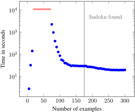
In this experiment we take a closer look at the runtime required by our method, as a function of the number of examples. We focus on the Sudoku problem and run the experiment with the number |E| of examples going from 0 to 300 by steps of 5. For each value, we run our method five times (with |E+|/|E| = 0.5) and report the average runtime. If any of the five runs reaches the 3-hour timeout, we ignore the others and simply report a timeout for the corresponding |E|.
Figure 1 shows our results. An optimal constraint network (in the sense of our objective function) is found rather quickly when the number of examples is either extremely small (5 to 15) or sufficiently large (75 or more). This is unsurprising because examples translate into hard clauses in our WEIGHTED PARTIAL MAX-SAT model: with very few examples the model is underconstrained, and with sufficiently many examples the search space becomes small. The transition appears to occur between 15 and 70 examples, where the solver systematically reaches the timeout. As we will see in the next experiment, for such values of |E| the accuracy of an optimal constraint network would be close to 0.5. This means that very long runtimes are only observed for training sets that are too small for our method to learn the target constraint network (independently of the computational resources available). For 170 examples or more, the optimal solution is the target Sudoku network and is found in less than 30 seconds.
Accuracy
In this experiment we vary the number |E| of examples from 75 to 300 by steps of 5, again with |E+|/|E| = 0.5 for all training sets. For each value |E|, we run our method 5 times on samples of |E| randomly generated examples. We then measure the accuracy of each of the 5 learned constraint networks using 2000 additional examples. We report the average accuracy as a function of |E| in Figure 2.
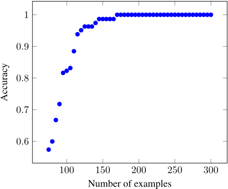
At 75 examples, the measured accuracy is close to 0.5, which means that the number of examples is too small to allow our method to learn a network capturing the problem. From 75 to 120 examples, the accuracy increases dramatically up to 0.95. From 120 to 170 examples the accuracy slowly increases up to 1. The slowness in winning these last percentage points of accuracy is explained by the fact that in this range, the learned constraint network is essentially a Sudoku model with a few additional difference constraints. As our method maximizes the number of constraints in the network, these extra constraints can only be ruled out a few at a time by positive examples. The accuracy reaches 1 at n = 170, at which point the target constraint network is found.
Ratio of Positive Examples
In this experiment, we vary the fraction of positive examples p = |E+|/|E| in the training set. For each p ∈ {0, 0.2, 0.4, 0.5, 0.6, 0.7, 0.8, 0.9, 1}, we generate training sets with a fraction p of positive examples. In Table 2 we report the minimum number of examples needed by our method to return the target Sudoku network. Results are averaged over five runs.
| p | 0 | 0.2 | 0.4 | 0.5 | 0.6 | 0.7 | 0.8 | 0.9 | 1 |
| |E| | × | 343 | 172 | 137 | 115 | 106 | 98 | 99 | × |
We observe that as the ratio of positive increases, fewer examples are needed to acquire the target network. This is not valid past a certain point because our method is not capable of learning the target constraint network with only positive examples. Indeed, in this case a degenerate constraint network with (k, r) = (1, 1) correctly classifies all examples and therefore will be returned. (Likewise, our method is incapable of learning the target network with p = 0.) We observe a slight increase in the number of required examples at p = 0.9 compared to p = 0.8, although the difference is within margin of error. Overall, it seems that our method performs best on the Sudoku problem when the ratio of positive examples is comprised between 0.6 and 0.9.
6 Conclusion
We proposed a constraint acquisition method that eliminates the need for advance knowledge of the target network's constraint language. Our method computes a suitable constraint language as part of the learning process, making it more widely applicable. Experiments are particularly encouraging, although they also highlight some limitations. We believe that some of these limitations (in particular, the fairly large number of examples sometimes required to win the last percentage points of accuracy and the difficulty to deal with large constraints languages) could be addressed in the future by integrating less rudimentary notions of simplicity than language size. Automatically detecting (or guessing) topological information about the target network, such as an eventual matrix structure, would also help greatly the learning process.
Acknowledgments
This work was partially supported by the TAILOR project, funded by EU Horizon 2020 research and innovation programme under GA No 952215, by the AI Interdisciplinary Institute ANITI, funded by the French program "Investing for the Future - PIA3" under grant agreement no. ANR19-PI3A-0004, and by the ANR AXIAUM project ANR20-THIA-0005-01 (Data Science Institute of the University of Montpellier). All the experiments have been performed with the support of MESO@LR-Platform at the University of Montpellier.
@inproceedings{ijcai2023p208,
  title     = {Learning Constraint Networks over Unknown Constraint Languages},
  author    = {Bessiere, Christian and Carbonnel, Clément and Himeur, Areski},
  booktitle = {Proceedings of the Thirty-Second International Joint Conference on
               Artificial Intelligence, {IJCAI-23}},
  publisher = {International Joint Conferences on Artificial Intelligence Organization},
  editor    = {Edith Elkind},
  pages     = {1876--1883},
  year      = {2023},
  month     = {8},
  note      = {Main Track},
  doi       = {10.24963/ijcai.2023/208},
  url       = {https://doi.org/10.24963/ijcai.2023/208},
}
TY - CPAPER TI - Learning Constraint Networks over Unknown Constraint Languages AU - Bessiere, Christian AU - Carbonnel, Clément AU - Himeur, Areski T2 - Proceedings of the Thirty-Second International Joint Conference on Artificial Intelligence, IJCAI-23 PB - International Joint Conferences on Artificial Intelligence Organization PY - 2023 SP - 1876 EP - 1883 DO - 10.24963/ijcai.2023/208 UR - https://doi.org/10.24963/ijcai.2023/208 ER -Copied
Machine-readable versions of this paper, for tools and AI agents:





