
Probabilistic Planning with Prioritized Preferences over Temporal Logic Objectives
Proceedings of the Thirty-Second International Joint Conference on Artificial Intelligence. Main Track. Pages 189-198.
https://doi.org/10.24963/ijcai.2023/22
Keywords
- Planning and Scheduling: PS: Markov decisions processes
- Knowledge Representation and Reasoning: KRR: Preference modelling and preference-based reasoning
- Agent-based and Multi-agent Systems: MAS: Formal verification, validation and synthesis
Abstract
This paper studies temporal planning in probabilistic environments, modeled as labeled Markov decision processes (MDPs), with user preferences over multiple temporal goals. Existing works reflect such preferences as a prioritized list of goals. This paper introduces a new specification language, termed prioritized qualitative choice linear temporal logic on finite traces, which augments linear temporal logic on finite traces with prioritized conjunction and ordered disjunction from prioritized qualitative choice logic. This language allows for succinctly specifying temporal objectives with corresponding preferences accomplishing each temporal task. The finite traces that describe the system's behaviors are ranked based on their dissatisfaction scores with respect to the formula. We propose a systematic translation from the new language to a weighted deterministic finite automaton. Utilizing this computational model, we formulate and solve a problem of computing an optimal policy that minimizes the expected score of dissatisfaction given user preferences. We demonstrate the efficacy and applicability of the logic and the algorithm on several case studies with detailed analyses for each.
- [Benferhat and Sedki, 2007] Salem Benferhat and Karima Sedki. A revised qualitative choice logic for handling prioritized preferences. In European Conference on Sym- bolic and Quantitative Approaches to Reasoning and Un- certainty, pages 635-647. Springer, 2007.
- [Benferhat and Sedki, 2008] Salem Benferhat and Karima Sedki. Two alternatives for handling preferences in qualitative choice logic. Fuzzy Sets and Systems, 159(15):1889-1912, August 2008.
- [Bertsekas and Yu, 2013] Dimitri P Bertsekas and Huizhen Yu. Stochastic shortest path problems under weak condi- tions. Lab. for Information and Decision Systems Report LIDS-P-2909, MIT, 2013.
- [Bradley et al., 2021] Christopher Bradley, Adam Pacheck, Gregory J Stein, Sebastian Castro, Hadas Kress-Gazit, and Nicholas Roy. Learning and planning for tempo- rally extended tasks in unknown environments. In 2021 IEEE International Conference on Robotics and Automa- tion (ICRA), pages 4830-4836. IEEE, 2021.
- [Brewka et al., 2004] Gerhard Brewka, Salem Benferhat, and Daniel Le Berre. Qualitative choice logic. Artificial Intelligence, 157(1):203-237, August 2004.
- [Cai et al., 2020] Mingyu Cai, Hao Peng, Zhijun Li, Hongbo Gao, and Zhen Kan. Receding horizon control-based mo- tion planning with partially infeasible ltl constraints. IEEE Control Systems Letters, 5(4):1279-1284, 2020.
- [Camacho et al., 2017] Alberto Camacho, Eleni Triantafil- lou, Christian Muise, Jorge A Baier, and Sheila A McIl- raith. Non-deterministic planning with temporally ex- tended goals: Ltl over finite and infinite traces. In Thirty- First AAAI Conference on Artificial Intelligence, 2017.
- [De Giacomo and Favorito, 2021] Giuseppe De Giacomo and Marco Favorito. Compositional approach to translate ltlf/ldlf into deterministic finite automata. In Proceedings of the International Conference on Automated Planning and Scheduling, volume 31, pages 122-130, 2021.
- [De Giacomo and Vardi, 2013] Giuseppe De Giacomo and Moshe Y Vardi. Linear temporal logic and linear dynamic logic on finite traces. In IJCAI'13 Proceedings of the Twenty-Third international joint conference on Artificial Intelligence, pages 854-860. Association for Computing Machinery, 2013.
- [De Giacomo and Vardi, 2015] Giuseppe De Giacomo and Moshe Vardi. Synthesis for ltl and ldl on finite traces. In Twenty-Fourth International Joint Conference on Artificial Intelligence, 2015.
- [Droste and Gastin, 2009] Manfred Droste and Paul Gastin. Weighted automata and weighted logics. In Handbook of weighted automata, pages 175-211. Springer, 2009.
- [He et al., 2015] Keliang He, Morteza Lahijanian, Lydia E Kavraki, and Moshe Y Vardi. Towards manipulation planning with temporal logic specifications. In 2015 IEEE international conference on robotics and automation (ICRA), pages 346-352. IEEE, 2015.
- [He et al., 2020] Binghan He, Jaemin Lee, Ufuk Topcu, and Luis Sentis. Bp-rrt: Barrier pair synthesis for temporal logic motion planning. In 2020 59th IEEE Conference on Decision and Control (CDC), pages 1404-1409. IEEE, 2020.
- [Hekmatnejad and Fainekos, 2018] Mohammad Hekmatne- jad and Georgios Fainekos. Optimal multi-valued ltl plan- ning for systems with access right levels. In 2018 Annual American Control Conference (ACC), pages 2363-2370. IEEE, 2018.
- [Kantaros et al., 2022] Yiannis Kantaros, Samarth Kallu- raya, Qi Jin, and George J Pappas. Perception-based tem- poral logic planning in uncertain semantic maps. IEEE Transactions on Robotics, 2022.
- [Kasenberg et al., 2020] Daniel Kasenberg, Ravenna Thiel- strom, and Matthias Scheutz. Generating explanations for temporal logic planner decisions. In Proceedings of the International Conference on Automated Planning and Scheduling, volume 30, pages 449-458, 2020.
- [Lacerda et al., 2015] Bruno Lacerda, David Parker, and Nick Hawes. Optimal policy generation for partially satis- fiable co-safe ltl specifications. In Twenty-Fourth Interna- tional Joint Conference on Artificial Intelligence, 2015.
- [Lahijanian and Kwiatkowska, 2016] Morteza Lahijanian and Marta Kwiatkowska. Specification revision for Markov decision processes with optimal trade-off. In Proc. 55th Conference on Decision and Control (CDC'16), pages 7411-7418, 2016.
- [Li et al., 2020] Meilun Li, Andrea Turrini, Ernst Moritz Hahn, Zhikun She, and Lijun Zhang. Probabilistic pref- erence planning problem for markov decision processes. IEEE transactions on software engineering, 2020.
- [Li et al., 2021] Shen Li, Daehyung Park, Yoonchang Sung, Julie A Shah, and Nicholas Roy. Reactive task and mo- tion planning under temporal logic specifications. In 2021 IEEE International Conference on Robotics and Automa- tion (ICRA), pages 12618-12624. IEEE, 2021.
- [Mallett et al., 2021] Ian Mallett, Sylvie Thiébaux, and Fe- lipe Trevizan. Progression heuristics for planning with probabilistic ltl constraints. In Proceedings of the AAAI Conference on Artificial Intelligence, volume 35, pages 11870-11879, 2021.
- [Mehdipour et al., 2021] Noushin Mehdipour, Cristian-Ioan Vasile, and Calin Belta. Specifying User Preferences Us- ing Weighted Signal Temporal Logic. IEEE Control Sys- tems Letters, 5(6):2006-2011, December 2021.
- [Pnueli, 1981] Amir Pnueli. The temporal semantics of concurrent programs. Theoretical computer science, 13(1):45-60, 1981.
- [Puterman, 2014] Martin L Puterman. Markov decision pro- cesses: discrete stochastic dynamic programming. John Wiley & Sons, 2014.
- [Rahmani and O'Kane, 2019] Hazhar Rahmani and Jason M O'Kane. Optimal temporal logic planning with cascad- ing soft constraints. In 2019 IEEE/RSJ International Con- ference on Intelligent Robots and Systems (IROS), pages 2524-2531. IEEE, 2019.
- [Rahmani and O'Kane, 2020] Hazhar Rahmani and Jason M O'Kane. What to do when you can't do it all: Tem- poral logic planning with soft temporal logic constraints. In 2020 IEEE/RSJ International Conference on Intelli- gent Robots and Systems (IROS), pages 6619-6626. IEEE, 2020.
- [Tumova et al., 2013a] Jana Tumova, Luis I Reyes Cas- tro, Sertac Karaman, Emilio Frazzoli, and Daniela Rus. Minimum-violation ltl planning with conflicting specifica- tions. In American Control Conference, pages 200-205. IEEE, 2013.
- [Tumova et al., 2013b] Jana Tumova, Gavin C Hall, Ser- tac Karaman, Emilio Frazzoli, and Daniela Rus. Least- violating control strategy synthesis with safety rules. In Proc. Int. Conf. on Hybrid systems: Computation and con- trol, 2013.
- [Vasile et al., 2017] Cristian-Ioan Vasile, Jana Tumova, Ser- tac Karaman, Calin Belta, and Daniela Rus. Minimum- violation scltl motion planning for mobility-on-demand. pages 1481-1488. IEEE, 2017.
- [Vasile et al., 2020] Cristian Ioan Vasile, Xiao Li, and Calin Belta. Reactive sampling-based path planning with tem- poral logic specifications. The International Journal of Robotics Research, 39(8):1002-1028, 2020.
- [Wang et al., 2020] Yu Wang, Siddhartha Nalluri, and Miroslav Pajic. Hyperproperties for robotics: Planning via hyperltl. In 2020 IEEE International Conference on Robotics and Automation (ICRA), pages 8462-8468. IEEE, 2020.
- [Wolper, 2001] Pierre Wolper. Constructing Automata from Temporal Logic Formulas: A Tutorial. In G. Goos, J. Hartmanis, J. van Leeuwen, Ed Brinksma, Holger Her- manns, and Joost-Pieter Katoen, editors, Lectures on For- mal Methods and PerformanceAnalysis, volume 2090, pages 261-277. Springer Berlin Heidelberg, Berlin, Hei- delberg, 2001.
- [Wongpiromsarn et al., 2021] Tichakorn Wongpiromsarn, Konstantin Slutsky, Emilio Frazzoli, and Ufuk Topcu. Minimum-violation planning for autonomous systems: Theoretical and practical considerations. In 2021 American Control Conference, 2021.
- [Yang et al., 2020] Yuanjiang Yang, Xiang Yin, and Shaoyuan Li. A distributed framework for multi-robot task planning with temporal logic specifications. In 2020 IEEE 16th International Conference on Control & Automation (ICCA), pages 570-575. IEEE, 2020.
- [Zhao et al., 2022] Jiawei Zhao, Xiang Yin, and Shaoyuan Li. Temporal logic robot task planning with active acquisi- tion of information. In 2022 IEEE 17th International Con- ference on Control & Automation (ICCA), pages 1014- 1020. IEEE, 2022.
- [Zhou et al., 2022] Xiaoyi Zhou, Tiange Yang, Yuanyuan Zou, Shaoyuan Li, and Hao Fang. Multiple sub-formulae cooperative control for multi-agent systems under conflict- ing signal temporal logic tasks. IEEE Transactions on In- dustrial Electronics, 2022.
References were extracted automatically from the PDF and may contain errors.
Full text extracted automatically from the PDF; figures, tables and equations may differ. The PDF is the version of record.
1 Introduction
In this work, we study preference-based planning given a preference order over temporal goals, i.e. , ordered goals specified in temporal logics . Temporal logics are expressive and rigorous languages for specifying complex tasks and mission objectives. Planning with temporal logic goals [Pnueli, 1981] has seen studied for robotic systems [Kantaros et al., 2022; Bradley et al., 2021; He et al., 2020; Vasile et al., 2020; Yang et al., 2020; Wang et al., 2020; Hekmatnejad and Fainekos, 2018; He et al., 2015; Li et al., 2021] and other intelligent systems [Kasenberg et al., 2020; De Giacomo and Vardi, 2015; Camacho et al., 2017; Mallett et al., 2021; Zhou et al., 2022; Zhao et al., 2022].
∗This material is based upon work supported by Air Force Office of Scientific Research under award number FA9550-21-1-0085 and by NSF under Grant No. 2024802 and Grant No.2144113.
Specifying preferences over temporal goals gives the decision maker some flexibility to revise the task and achieve the most preferred outcomes when not all constraints/subtasks can be satisfied. Early works consider deterministic systems-modeled as finite, discrete systems or system with deterministic dynamics. Several works [Tumova et al., 2013b; Tumova et al., 2013a; Wongpiromsarn et al., 2021; Vasile et al., 2017] proposed minimumviolation planning methods, that decide which low-priority constraints should be violated. [Mehdipour et al., 2021] associate weights with Boolean and temporal operators in signal temporal logic to specify the importance of satisfying the subformula and priority in the timing of satisfaction. They develop algorithms to maximize the weighted satisfaction in deterministic dynamical systems. [Rahmani and O'Kane, 2019; Rahmani and O'Kane, 2020] studied temporal planning given both hard and soft specifications of the goal, using linear temporal logic (LTL) and linear dynamic logic on finite traces (LDLf ). [Cai et al., 2020] consider minimizing the deviations from infeasible LTL specifications while maximizing the total rewards.
Several recent works study preference-based probabilistic planning with temporal logic goals. [Li et al., 2020] consider preference-based planning for Markov decision process (MDP) subject to an ordered list of probabilistic temporal logic formula. The algorithm enumerates the tasks one by one in a prioritized order until a policy that satisfies the most preferred task is found. [Lahijanian and Kwiatkowska, 2016] studied syntactically co-safe LTL planning with infeasible specifications in environments modeled by MDPs. They compute a policy that maximizes the probability of satisfying a revised formula and minimizes the cost of revision. [Lacerda et al., 2015] considered a similar problem where the aim is to synthesize a policy that, in decreasing order of priority, maximizes the probability of completing the task, maximizes the probability of progressing toward completion, and minimizes the expected cost.
Despite the existing work on probabilistic preferencebased planning, the connection between preference specification in AI and preferences over temporal goals is yet to be established. We propose a new language that extends temporal logic with fuzzy logic representation of preferences. Specifically, we consider qualitative choice logic (QCL) proposed by [Brewka et al., 2004] and its extension prioritized qualitative choice logic (PQCL) [Benferhat and Sedki, 2007; Benferhat and Sedki, 2008]. QCL extends propositional logic with a new logical connective called ordered disjunction, denoted →×. Formula A →× B means if possible then A, but if A is not possible then at least B. PQCL introduced prioritized conjunction/disjunction to QCL by allowing the user to express priorities in a user's preference. Combined, if (A →× B)&(C →× D) where & is the prioritized conjunction, then the preference of A →×B is more important to be satisfied than the preference C →× D.
The preference language proposed herein, called prioritized qualitative choice linear temporal logic on finite traces (PQCLTLf ), integrates PQCL with a subclass of LTL over finite traces. In particular, we introduce LTL formulas for atomic preference and employ PQCL to represent a preference over the temporal goals. We assign a dissatisfaction score for each outcome (temporal sequence of states) in light of semantics for PQCL. This scoring function enables us to formulate a preference-based probabilistic planning objective, that is, to minimize the expected dissatisfaction score in a stochastic system, modeled as a labeled MDP.
However, this compact, logical representation of preferences alone is not sufficient for probabilistic planning, which generally requires a computational model. Based on the relation between LTL and automata, we develop a procedure that translates a PQCLTLf formula into a weighted deterministic finite automaton. This weighted automaton ensures for each path that satisfies the preference to a degree k, the sum of weights of the corresponding induced run on the weighted automaton is exactly k. Augmenting the planning state space with the state set of the weighted automata using a product operation, we show that the most preferred policy in the stochastic system can be obtained by solving a product MDP. The correctness of the solution hinges upon the definition of a reward function based on the weights on transitions in the weighted automaton. We formally prove that the rewardmaximizing policy in the product MDP minimizes the expected degree of dissatisfaction in the original MDP given the PQCLTLf formula. In our experiments, we employ several robotic motion planning examples to demonstrate the efficacy and applicability of the method and provide a detailed comparison of preference-based planning and traditional planning with a monolithic temporal logic formula.
2 Preliminaries
Notations. The set of all probability distributions over a finite set X is denoted D(X).
We introduce necessary preliminaries and notations next.
Systemmodel. We model the interaction between the planning agent (a robot) and its stochastic environment as a variant of MDP.
Definition 1 (Labeled Markov Decision Process with a terminating state). A labeled Markov decision process with a teminating state (TLMDP) is a tuple M = 〈S,A := ∪s∈SAs, P, s0, s⊥, AP, L〉 where S is a finite set of states; A
is a finite set of actions, where for each state s ∈ S, As is the set of available actions at s; A includes a special terminating action a⊥ and for any s ∈ S, a⊥ ∈ As. P : S × A → D(S) is the transition probability function, where for each s, s′ ∈ S and a ∈ A, P(s′ | s, a) is the probability that the MDP transitions to s′ after taking action a at s; s0 ∈ S is the initial state; s⊥ ∈ S is the terminating state, which is a unique sink state. For any s ∈ S, P(s, a⊥, s⊥) = 1. That is, if an agent selects the terminating action a⊥, then a terminating state s⊥ can be reached surely. The set AP is a finite set of atomic propositions; and L: S → 2AP ∪ {⋉} is a labeling function that assigns to each state s ∈ S \ {s⊥}, the set of atomic propositions L(s) ⊆ AP that hold in s. Only the terminating state is labeled the "ending" symbol ⋉, i.e., L(s⊥) = ⋉.
A finite run in this MDP is a sequence ϱ = s0a0s1a1 · · · sk-1ak-1sk, in which, s0 is the initial state and for each 0 ≤ i ≤ k - 1, P(si+1 | si, ai) > 0. The path associated with this run is the sequence ρ = s0s1 · · · sk ∈ S∗ an the trace of this path is defined as trace(ρ) = L(s0)L(s1)L(s2) · · · L(sk) ∈ (2AP )∗ . A path which ends at s⊥ is called terminating.
A finite-memory, randomized policy in the MDP is a function π : S∗ → D(A) that maps a state sequence into a distribution over actions. A Markovian, or memoryless, randomized policy in the MDP is a function π : S → D(A) that maps the current state into a distribution over actions. We denote the set of all randomized policies as Π.
A finite-memory, randomized policy π : S∗ → D(A) induces a Markov chain M π = 〈S∗ , P π 〉 over S∗ as follows: For any ρ ∈ S∗ , s ∈ S,
where Last(ρ) is the last state given the sequence ρ, and π(ρ, a) denotes the probability of selecting action a under the path ρ given the policy π.
The stochastic process induced by a Markov policy is a Markov chain M π = 〈S∗ , P π 〉, where P π can be obtained as a special case of (1). The probability of a path ρ in the Markov chain M π is denoted by Pr(ρ;M π ).
Planning objectives. We are interested in probabilistic planning subject to a preference over a set of goals expressed using linear temporal logic on finite traces (LTLf ) formulas.
Definition 2 (LTLf Syntax [De Giacomo and Vardi, 2013]). Given a finite set AP of atomic propositions, the syntax of LTLf formulas is defined as follows:
where p ∈ AP, negation (¬) and conjunction (∧) are standard Boolean operators, and "Next" (©) and "Until" (U) are temporal operators.
Informally, formula ©ϕ states that ϕ holds at the next time instant, and ϕ1 Uϕ2 means there is a future time instant at which ϕ2 holds and for all time instants from the current time until that future time, ϕ1 holds true. The temporal operator "Eventually" (♦ ) is defined using "Until" as ♦ ϕ := true U ϕ. The dual of this operator is "Always" (□), which is defined as □ϕ := ¬♦¬ϕ. Formula ♦ϕ means there is some future time instant at which ϕ holds, while □ϕ is interpreted that ϕ is true at the current instant and all future instants. The semantics of LTLf is given as interpretations over finite traces and can be found in [De Giacomo and Vardi, 2013].
The language of an LTLf formula ϕ, denoted L(ϕ), is the set of words over the alphabet 2AP that satisfy ϕ. For notation simplicity, let Σ := 2AP in the following context. The set of all finite words over a finite alphabet Σ is denoted by Σ∗ . The language of LTLf formula ϕ can be represented by the set of words accepted by a deterministic finite automaton (DFA) Aϕ = 〈Q, Σ, δ, q0, F〉, where Q is a finite set of states; Σ = 2AP is the alphabet; δ : Q×Σ → Q is a transition function such that δ(q, σ) = q′ is the state reached upon reading input σ from state q; q0 ∈ Q is an initial state; and F ⊆ Q is a set of accepting/final states. A transition function is recursively extended in the general way: δ(q, σw) = δ(δ(q, σ), w) for a given σ ∈ Σ and w ∈ Σ∗ . A word w is accepting if and only if δ(q,w) ∈ F. The DFA Aϕ accepts the exact set of words satisfying ϕ given the semantics of LTLf .
3 Preference Language: Integration of Prioritized Qualitative Choice Logic and Temporal Logic
In this section, we present a new task specification language to describe a subset of preferences over temporal goals. We call this language PQCLTLf , which combines LTLf with PQCL [Benferhat and Sedki, 2007]-a propositional logic for representing ranked objectives.
PQCL augments propositional logic with a connective →×, called ordered disjunction: A formula φ1 →× φ2 means that if possible then φ1, and if φ1 is not possible then φ2. The operator →× is left-associative, and therefore φ1 →× φ2 →×. . . →×φn = φ1 →× (φ2 →×(. . . →×φn) . . .). In addition to ordered disjunction, PQCL introduces prioritized conjunction: A formula φ1&φ2 defines the lexicographical ordering between individual satisfaction of φ1 and φ2.
Definition 3 (Prioritized Qualitative Choice Linear Temporal Logic on Finite Traces). Let Φ be a set of LTLf formulas over a set AP of atomic propositions. A PQCLTLf fragment over AP (without negation) is defined by
in which ψ ∈ Φ.
In comparison to PQCL, we do not include negation operation and thereby exclude the prioritized disjunction. Negation is only allowed in the construction of LTLf formulas. The reason of not including negation is mainly due to ambiguity:
A negation of flight→×train can mean the two options are indifferent, incomparable, or train is preferred to flights. To avoid confusion, the indifference between "flight" and "train" can be expressed as regular disjunction in LTLf and the preference of "train" to "flight" can be expressed as train →× flight. The PQCLTLf does not consider incomparable options.
The optionality [Benferhat and Sedki, 2007] of a PQCL formula defines how many ways the formula can be satisfied. Likewise, we have the following definition of optionality of a PQCLTLf formula.
Definition 4 (Optionality, extended from [Benferhat and Sedki, 2007]). Given an PQCLTLf formula ϕ, the optionality of ϕ, denoted opt(ψ), is the number of ways ϕ can be satisfied, and is computed recursively as follows:
- If ϕ is an LTLf formula, then opt(ϕ) = 1;
- If ϕ = ϕ1 →× ϕ2, then opt(ϕ) = opt(ϕ1) + opt(ϕ2);
- If ϕ = ϕ1&ϕ2, then opt(ϕ) = opt(ϕ1) · opt(ϕ2).
Associated with this definition of optionality, for each word w ∈ Σ∗ and a PQCLTLf formula ϕ, w satisfies ϕ to a certain degree.
Definition 5 (Satisfaction Degree, extended from [Benferhat and Sedki, 2007]). Let ϕ be a PQCLTLf formula over AP and w ∈ Σ∗ (recall Σ = 2AP ) be a finite word. We write w |=k ϕ for some positive integer k > 0 to denote that the satisfaction degree of w with respect to ϕ is k, and use w ̸|= ϕ to denote that w does not satisfy ϕ.
The satisfaction degree of w with respect to ϕ is computed as follows:
- If ϕ is an LTLf formula, then w |=1 ϕ if w ∈ L(ϕ), and w ̸|= ϕ if w ̸∈ L(ϕ).
- If ϕ = ϕ1 →×ϕ2, then w |=k ϕ1 →×ϕ2 if
- either w |=k ϕ1; or
- w |=n ϕ2, w ̸|= ϕ1, and k = n + opt(ϕ1).
Otherwise, if w ̸|= ϕ1 and w ̸|= ϕ2, then w ̸|= ϕ1 →× ϕ2.
- If ϕ = ϕ1&ϕ2, then w |=k ϕ1&ϕ2 if there exist i, j > 0 such that w |=i ϕ1, w |=j ϕ2, and k = opt(ϕ2) × (i - 1) + j; otherwise, if w ̸|= ϕ1 or w ̸|= ϕ2, then w ̸|= ϕ1&ϕ2.
The definition of satisfaction degree induces a total order only on the set of all the words that satisfy the PQCLTLf formula, but it does not rank those words who do not satisfy the formula. For planning purposes, we introduce a metric whose range of values is circumscribed between 0 and 1.
Definition 6 (Dissatisfaction Score). The dissatisfaction score function is a function d : Σ∗ × Φ → (0, 1] that assigns to each word w ∈ Σ∗ and PQCLTLf formula ϕ ∈ Φ, a positive real value in (0, 1], called the dissatisfaction score of w with respect to ϕ, which is computed as follows:
- If w ̸|= ϕ, then d(w, ϕ) = 1;
- If w |=k ϕ for k > 0, then d(w, ϕ) = k opt(ϕ)+1 .
The lower the score, the more satisfied is the word. Note that the score is always greater than 0. In the following context, when the formula ϕ is clear from the context, we simply write d(w) for the dissatisfaction score of w w.r.t. ϕ.
Each PQCLTLf formula ϕ over a set of atomic propositions AP induces a preference model ⪰ϕ over Σ∗ such that for any two words w, w′ ∈ Σ∗ , w is preferred to w′ with respect to ϕ, i.e. , w ⪰ϕ w′ , if and only if d(w, ϕ) ≤ d(w′ , ϕ).
It is easy to prove the following property.
Lemma 1. If w ⪰ϕ w′ , then one of the following conditions holds: 1. w |=k ϕ and w′ ̸|= ϕ; or 2. w |=n ϕ, w′ |=m ϕ, and n ≥ m.
The preference model over Σ∗ directly translates to a preference model over S∗-the set of finite paths in a labeled MDP-such that path ρ ∈ S∗ is preferred to ρ′ ∈ S∗ if and only if d(L(ρ), ϕ) ≤ d(L(ρ′ ), ϕ). Thus, given a policy in a labeled MDP, we introduce the following measure to evaluate how preferred a policy is with respect to a PQCLTLf formula.
Definition 7 (Expected Dissatisfaction Score). Let π be a finite-memory, randomized policy for a given MDP, M π = 〈S∗ , P π 〉 be its induced Markov chain, and ϕ be a PQCLTLf formula. The expected dissatisfaction score of π with respect to ϕ, denoted by d(π, ϕ), is defined
We now formally state the probabilistic planning problem:
Problem [Probabilistic Planning with Prioritized Preferences over Temporal Logic Objectives (PrefTL-MDP)]:
Given a labeled MDP M = 〈S,A := ∪s∈SAs, P, s0, s⊥,AP,L〉 and a PQCLTLf formula ϕ, compute a policy π: S∗ → D(A) that minimizes the expected dissatisfaction score of ϕ .
4 Optimal Planning for PQCLTLf Formulas
We now present a planning algorithm to solve the PrefTLMDP problem. Our approach consists of two steps: In the first step, we construct an automata-theoretic model for PQCLTLf formula. In the second step, we show that the optimal policy that minimizes the expected dissatisfaction score of the given formula can be computed by solving a rewardmaximizing MDP with augmented states.
4.1 Automata-Theoretic Modeling of PQCLTLf Formulas
In this section, we focus on constructing a computational model for a given prioritized qualitative choice temporal logic (PQCTL) formula ϕ. The choice of such a computational model for representing the subclass of PQCLTLf formulas is a weighted deterministic finite automaton.
Definition 8 (Weighted Deterministic Finite Automaton [Droste and Gastin, 2009]). A weighted deterministic finite automaton is a tuple A = 〈Q, Σ, δ, q0, w〉, where Q is a finite set of states; Σ ∪ {⋉} is a finite set of symbols (alphabet); and ⋉ is a unique symbol representing the end of a string 1 ; δ : Q × (Σ ∪ {⋉}) → Q is a deterministic transition function; q0 is the initial state; and w : Q×(Σ∪{⋉})×Q→R is a weight function that assigns each transition (q, σ, q′ ) to a real value, called the weight of this transition.
1 In general, one can include ⋊ as the beginning of a finite string and ⋉ as the ending of a finite string. The beginning symbol ⋊ is omitted as it is clear from the context.
Consider a finite word w = σ0σ1 . . . σn-1⋉, let w[i] be the i-th symbol of this word. The run ρ generated by word w is ρ := q0σ0q1 . . . σn-1qn that satisfies qi+1 = δ(qi, w[i]), for i = 0, . . . , n - 1. We write Word(ρ) = w to denote the word associated with the run ρ. The total weight is w(ρ) = ∑n-1 i=0 w(qi, w[i], qi+1).
First, we show how to construct the weighted deterministic finite automaton (WDFA) for a LTLf formula ϕ.
Definition 9 (WDFA for an LTLf Formula ϕ). Let Aϕ = 〈Q, Σ, δ, q0, F 〉 be a DFA encoding ϕ. A WDFA for encoding ϕ is constructed from Aϕ as a tuple
in which for each q ∈ Q ∪ {sink} and σ ∈ Σ ∪ {⋉},
and for each q, q′ ∈ Q ∪ {sink} and σ ∈ Σ ∪ {⋉},
Intuitively, the WDFA A extends the DFA Aϕ with a sink state sink. For any state s ∈ S of the original DFA Aϕ, a transition to sink is made with an input symbol ⋉. A weight one is received only if the transition is from an accepting state to the sink state upon reading the ending symbol ⋉.
Lemma 2. Given a WDFA A for an LTLf formula ϕ and a finite run ρ = q0σ0q1 . . . σn-1qn, if w(ρ) = 1 then Word(ρ) |=1 ϕ.
The proofs of Lemmas 2, 3 4, and 5 can be found in Appendix A.1. Next, we define the construction process of WDFAs for ordered disjunction and prioritized conjunction of PQCLTLf formulas.
Definition 10 (WDFA for Ordered Disjunction of PQCLTLf Formulas). Let Ai = 〈Qi ∪ {sinki},Σ ∪ {⋉}, δi, q0i,wi〉 for i = 1, 2 be two WDFA's that respectively encode two PQCLTLf formulas ϕ1, ϕ2. One can constrcut from them, a WDFA for ϕ1 →× ϕ2 as a tuple A = 〈Q1 × Q2 ∪ {sink}, Σ ∪ {⋉}, δ, (q01, q02),w〉, in which, the transition function is defined as, for any (q1, q2) ∈ Q1 × Q2 and σ ∈ Σ ∪ {⋉},
and the weight function is defined as,
Lemma 3. Given a WDFA A for ϕ = ϕ1 →× ϕ2 and a finite run ρ = q0σ0q1 . . . qn-1σn-1qn, if w(ρ) = k for a k > 0, then Word(ρ) |=k ϕ, else Word(ρ) ̸|= ϕ.
Definition 11 (WDFA for Prioritized Conjunction of PQCLTLf Formulas). Let Ai = 〈Qi ∪ {sinki},Σ ∪ {⋉}, δi, q0i,wi〉 for i = 1, 2 be two WDFA's that respectively encode two PQCLTLf formulas ϕ1, ϕ2. One can construct from them, a WDFA for ϕ1&ϕ2 as a tuple A = 〈Q1 × Q2 ∪ {sink}, Σ ∪ {⋉}, δ, (q01, q02), w〉, in which, the transition function is defined as, for any (q1, q2) ∈ Q1 ×Q2 and σ ∈ Σ ∪ {⋉},
and the weight function is defined as,
- For any (q1, q2) ∈ Q1 ×Q2, for σ ∈ Σ, w((q1, q2), σ, (δ1(q1, σ), δ2(q2, σ))) = 0
- For any (q1, q2) ∈ Q1 × Q2, for input ⋉, if wi(qi, ⋉, sink) > 0 for both i = 1, 2, then
Lemma 4. Given a WDFA A for ϕ = ϕ1&ϕ2, and a finite run ρ = q0σ0q1 . . . qn-1σn-1qn, if w(ρ) = k for a k > 0, then Word(ρ) |=k ϕ, else Word(ρ) ̸|= ϕ.
Given the above construction methods of WDFAs for PQCLTLf formulas, the WDFA for a more complex PQCLTLf formulas can be constructed recursively.
Lemma 5. Given a PQCLTLf formula ϕ for which L(ϕ) ̸= ∅ and the constructed WDFA A, the optionality of ϕ is the maximal weight of all transitions in A. That is,
An example to illustrate the construction of WDFAs is given in the Appendix A.2.
5 Probabilistic Planning toMinimize the Dissatisfaction Score
In this section, we show how to leverage the WDFA for solving Problem PrefTL-MDP. Similar to probabilistic planning with linear temporal logic constraints, a product operation between the labeled MDP and the WDFA allows us to keep track of temporal objectives.
Definition 12 (The product between the labeled MDP and a WDFA). The product of a given WDFA A = 〈Q∪{sink}, Σ∪ {⋉}, δ, q0, w〉 and a terminating labeled MDP M = 〈S, A := ∪s∈SAs, P, s0, s⊥, AP, L〉 is an MDP
in which
- V = S ×Q is the state space,
- A is the set of actions, and for each v = (s, q) ∈ V , Av = As is the set of available actions at state v,
- P is the probabilistic transition function, where for each states (s, q), (s′ , q′ ) ∈ V and action a ∈ A,
- v0 = (s0, δ(q0,L(s0))) is the initial state.
- R : V ×A → R is the reward function, where for each (s, q) ∈ V and a ∈ A, if a = a⊥ and w(q, ⋉, sink) > 0, then R((s, q), a⊥) = opt(ϕ) - w(q, ⋉, sink) + 1, else R((s, q), a) = 0.
Given a finite run h = v0a0v1a1 . . . vn in the product MDP, the total reward is R(h) = ∑n-1 i=0 R(vi, ai). Since a run h in the product MDP corresponds to a run ρ in the original MDP except that each state in ρ is augmented with an automaton state, we use ProjS(h) to compute the projection of the run h = (s0, q0)(s1, q1) . . . (sn, qn) ∈ V ∗ to a run s0s1s2 . . . sn ∈ S∗ , whose labeling is L(s0s1 . . . sn) = L(s0)L(s1) . . . L(sn). We denote the set of finite runs inM by Runs(M).
Based on the reward function, the expected total reward of a nonstationary policy π : V ∗ → D(A) for an initial state v ∈ V is defined as
with Jπ,N(v) being the expected N-stage reward of π for state v:
where Vk is the state at time k. The expectation is with respect to the distribution of paths in the stochastic process Mπ .
Lemma 6. For any policy π : V ∗ → D(A) of the product MDPM, for any v ∈ V , Jπ(v) <∞.
The proof is in Appendix A.1.
The optimal value function is defined to be
For optimal planning to maximize the total reward, J ∗ (v) can be attained by a Markovian policy [Puterman, 2014]. Therefore, in the following, we only consider Markovian policies. We also consider the Bellman operator T , defined by
and the optimal value function satisfies TJ ∗ = J ∗ .
Among all the Markovian policies for the product MDP, we consider only the proper ones.
Definition 13 (Extended from [Bertsekas and Yu, 2013]). A policy π for the MDP M is proper if it guarantees that the sink state (s⊥, sink) will be reached with probability one.
Lemma 7. The optimal value J ∗ (v) for any v ∈ V can be obtained by a proper, Markovian policy of product MDP M.
The proof is in Appendix A.1.
Thus, to search an optimal policy, we need to consider only proper, Markovian policies. We now relate the reward maximizing problem in the product MDP to the planning objective of minimizing the expected dissatisfaction score.
Lemma 8. For each path h = (s0, q0)(s1, q1) . . . (sn, qn) ∈ V ∗ , it holds that,
The proof is in Appendix A.1.
Theorem 1. Let π : V → D(A) be a policy for the product MDP M. Construct from π, a policy π′ : S∗ → D(A) for M such that for each ρ = s0s1 · · · sn ∈ S∗ , π′ (ρ) = π((sn, δ(q0, L(ρ)))). If π is an optimal policy forM, then π′ is an optimal policy that minimizes the expected dissatisfaction score, i.e. , the solution to PrefTL-MDP.
Proof. We establish a connection between the expected dissatisfication score of π′ and the value of π. First, we use (2) to expand the expected dissatisfication score of π′ :
Next, we expand the value of π.
Using the result of Lemma 8, we write this summation as:
replacing (opt(ϕ) + 1) by K and Pr(h;Mπ ) by Prπ (h),
From (7) to (8), we use the probability axiom that ∑h∈V ∗ Pr(h;Mπ ) = 1. From (8) to (9), we use Lemma 8 that if R(h) = 0 then d(L(ProjS(h))) = 1. Thus, relating (9) and (5), we haveJπ(v0) = K - K · d(π′ , ϕ), (10)
and therefore argmaxπ Jπ(v0) = argminπ′ d(π′ , ϕ), that is, a policy π that maximizes J yields a policy π′ that minimizes the dissatisfaction score d.
6 Complexity Analysis
The first step of the algorithm constructs a WDFA that encodes ϕ. The constructed DFA from LTLf formulas is double-exponential in the size of the formulas in the worst case [Wolper, 2001; De Giacomo and Favorito, 2021]. However, in practice this translation is tractable for commonly seen LTLf formulas in robotic planning. The construction of automata for ordered disjunction ϕ1 →× ϕ2 and prioritized conjunction ϕ1&ϕ2 using Def. 10 and Def. 11 takes a polynomial time to the sizes of the WDFA's for sub-formulas ϕ1 and ϕ2, following the same complexity of computing the intersection of two DFAs. Constructing the product MDP M takes a polynomial time to the size of the WDFA and the MDP. And computing an optimal policy for M takes a time polynomial in the size of the product MDPM, with standard techniques (value/policy iteration or linear programming).
7 Experiment
We show the efficacy of the proposed algorithm using several examples of probabilistic robotic motion planning. 2
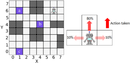
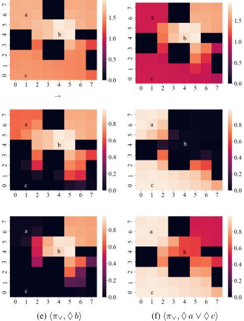
Consider a small stochastic gridworld g1 shown in Fig. 1. For each state s ∈ S, the robot has four actions: "N", "W", "S", "E". After taking an action from a state, the robot transits to the intended cell with probability 0.8 and slips to unintended cells with probability 0.1. If the robot takes an action and reaches the boundary wall, then it stays in the original cell. The initial state of the robot is (6, 6). The shaded areas denote holes. Once the robot enters a hole, it gets stuck. Regions of interest are labeled a, b, and c. Accordingly, AP = {a, b, c}. Each of these atomic propositions holds at a time instant when the robot is in the region labeled by the corresponding atomic proposition. Given the set AP of atomic propositions, we consider the following formula (see Appendix A.2 for the WDFA.): ♦b →× (♦a ∨ ♦c). We computed the optimal policy π∗ that minimizes the expected dissatisfaction score. To see the difference of ordered disjunction and regular disjunction, we also compute a optimal policy that maximizes the probability of satisfying formula ♦b ∨ (♦a ∨ ♦c). We denote this policy as π∨. We plot the optimal values for different initial states in Fig 2b. Then we perform policy evaluation of π∗ and π∨ against ♦b and ♦a ∨ ♦c, separately. The probabilites of satisfying formula φ for φ ∈ {♦ b, ♦ a∨♦ c} for different initial states are shown in Fig. 2c, 2d, 2e and 2f. Comparing Fig. 2c against Fig. 2e for the formula ♦b, π∗ achieves higher values in the most areas of the gridworld, especially at the top left corner. On the other side, comparing Fig. 2d against Fig. 2f, we can see that π∨ achieves higher probability of satisfying ♦a ∨ ♦c than that of policy π∗ in most areas of the gridworld, especially at the top right corner. This comparison indicates that when ♦b is preferred to ♦a ∨ ♦c, the preference-based policy gravitates towards satisfying ♦b. Next, we consider the following formula that has prioritized conjunction and nested ordered disjunctions: ϕ3 = ϕ1&ϕ2, where ϕ1 = ♦b →× (♦a ∨ ♦c) and ϕ2 = ♦(a∧♦(b∧♦c)) →×♦(a∧♦c)∨♦(b∧♦c). This task formula describes that the system needs to satisfy ϕ1 and ϕ2 both, with ϕ1 having a higher priority than ϕ2.
2 All experiments are executed on an Ubuntu 20.04 machine with AMD Ryzen 9 5900X CPU and 32 GB RAM. We use the Gurobi solver for planning in MDP. The computational times of solving the optimal planning problem for any 8 × 8 gridworlds with different formulas are no more than 0.1 seconds. The code can be found on github: https://github.com/leelening/ Plan-with-qualitative-choice-temporal-logic.
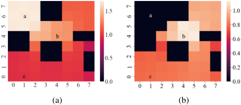
For this case, we consider an additional gridworld g2 which includes an additional hole at the position (2, 5), which blocks the access to a. Given the formula ϕ3, we compute the optimal policies π‡ when region a is accessible and π‡ when region a is inaccessible. We plot the heatmaps of ϕ3 for these two gridworlds in Fig. 3a and 3b. The following observation is made: When a is accessible, starting from the upper left corner, the agent receives higher values with the optimal policy. But if a is not accessible, the upper left corner states have values zero. This is because the formulas ϕ2 cannot be satisfied as the agent cannot reach region c when starting from the upper left corner. Therefore, ϕ3 is not satisfiable. The state values under the optimal policy given a accessible are higher than the state values when a is not accessible, indicating the agent can achieve a more preferred outcome in the gridworld g1.
8 Conclusion
In this paper, we introduced a specification language, termed prioritized qualitative choice linear temporal logic on finite traces (PQCLTLf ), for compactly specifying a temporal goal along with the user's preferences on sub-goals. We presented an automatic translation from this language to weighted deterministic finite automaton. We used this translation in solving the problem of computing a policy that minimizes the expected dissatisfaction score of a given PQCLTLf formula in a stochastic environment modeled by an MDP. By bridging the gap between preferences in AI and temporal logic planning, this work enables future study that incorporates preference elicitation and learning from positive/negative data and adaptive planning in sequential decision-making problems.
A Appendix
A.1 Proofs
Proof of Lemma 2
Proof. The run ρ has a weight 1 if and only if qn-1 ∈ F, σn-1 = ⋉, and qn = sink. Due to the acceptance condition for DFAs, the word Word(ρ) = σ0σ1 . . . σn-1 is accepted and thus satisfies the LTLf formula ϕ.
Proof of Lemma 3
Proof. Given the penultimate state qn-1 = (q1, q2), if w1(q1, ⋉, sink) = w2(q2, ⋉, sink) = 0, then Word(ρ) ̸|= ϕ, meaning it does not satisfy ϕ. If w1(q1,⋉, sink) = 0, but w2(q2,⋉, sink) > 0, then Word(ρ) satisfies ϕ2 to a positive degree but does not satisfy ϕ1. The satisfaction degree w.r.t. ϕ1 →× ϕ2 is the sum of the satisfaction degree w.r.t. ϕ2 and the optionality of ϕ1. Else, if w1(q1,⋉, sink) > 0, then the satisfaction degree w.r.t. ϕ1 →× ϕ2 is the satisfaction degree w.r.t. ϕ1.
Proof of Lemma 4
Proof. The proof is by construction and similar to the proof of Lemma 3. Thus, it is omitted.
Proof of Lemma 5
Proof. The property can be shown based on the recursive definition. First, it is clear that if the PQCLTLf formula is an LTLf formula, then the optionality is one and the maximal weight of all defined transitions is one. Consider two PQCLTLf formulas ϕ1, ϕ2, and their corresponding WDFAs A = 〈Qi ∪{sink}, Σ∪{⋉}, δi, q0i, wi〉 that satisfies opt(ϕi) = max{wi(q, a, q′ ) | δi(q, a, q′ ) is defined.}.
In the WDFA of the ordered disjunction ϕ1 →× ϕ2, the maximal weight by construction is max{w2(q2,⋉, sink) + opt(ϕ1)} = max{w2(q2, ⋉, sink)} + opt(ϕ1) = opt(ϕ2) + opt(ϕ1), which is consistent with Def. 4.
In the WDFA of the prioritized conjunction ϕ1&ϕ2, the maximal weight by construction is maxi,j{opt(ϕ2) × (i - 1) + j} where 0 < i ≤ max{w1(q1,⋉, sink)} = opt(ϕ1) and 0 < j ≤ max{w2(q2,⋉, sink)} = opt(ϕ2). Therefore, maxi,j {opt(ϕ2) × (i - 1) + j} = opt(ϕ2) × (opt(ϕ1) - 1) + opt(ϕ1) = opt(ϕ2) × opt(ϕ1). This is again consistent with Def. 4.
Proof of Lemma 6.
Proof. A finite run ρ = v0a0v1a1 . . . vn receives a nonzero reward only if there exists 0 ≤ k ≤ n, vk = (s⊥, sink), and for all j ≤ k, vj ̸= (s⊥, sink). The total reward of ρ is upper bounded by opt(ϕ). Therefore, for any policy π and any state v, the limit of Jπ,N(v) as N → ∞ exists and is upper bounded by opt(ϕ).
Proof of Lemma 7.
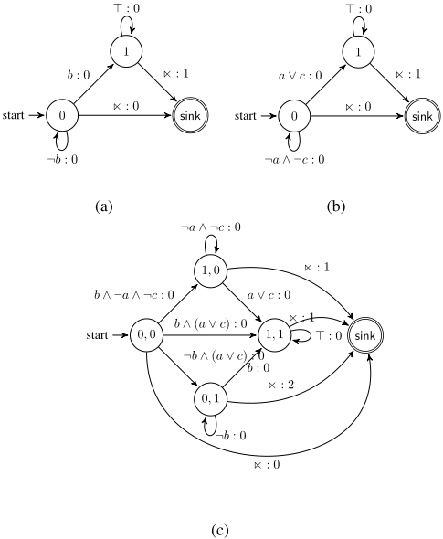
Figure 4: (a) The WDFA accepting the formula ♦ b. (b) The WDFA accepting the formula ♦a ∨ ♦c. (c) The WDFA accepting the formula ♦ b →× (♦ a ∨ ♦ c).
Proof. We show that for every improper, optimal Markovian policy, there is a proper, Markovian policy that obtains the same value. Consider an improper, optimal Markovian policy π† under which there is an infinite run. Since the reward is only obtained by reaching state (s⊥, sink), the infinite run h will have a reward of zero. Thus, a proper policy π∗ that has the same value Jπ† (v) = Jπ∗ (v) can be constructed by copying π† for all finite runs. For all infinite runs, π∗ is obtained from π† by terminating at any state with a zero reward.
Proof of Lemma 8.
Proof. Prove by construction. For the first case, let us recall R(h) = ∑n-1 i R(vi, ai). If L(ProjS(h)) |=k ϕ for some k > 0, then R(h) = opt(ϕ) -w(qn,⋉, sink) + 1. Plug in R(h), and we have d(L(ProjS(h)), ϕ) = 1 - R(h) opt(ϕ)+1 = w(qn,⋉,sink) opt(ϕ)+1 , complying with Lemma 2, 3, and 4. For the second case, if L(ProjS(h)) ̸|= ϕ, then R(h = 0), then d(L(ProjS(h)) = 1, complying with Def. 6.
A.2 Example of Weighted Automata Construction We illustrate the construction of WDFA using an example.
Example 1. Given two LTLf formulas ♦b and ♦a∨♦c and a PQCLTLf formula ♦b →× (♦a ∨ ♦c), reading "if possible, eventually satisfy b, and if not possible, eventually satisfy a or c." The WDFAs for the LTLf formulas are shown in Fig. 4a and 4b, and the WDFA is shown in Fig. 4c. For clarity, we use propositional logic formulas instead of 2AP as the symbols for the transitions. For example, b ∧ (a ∨ c) : 0 stands for {b, a} : 0, {b, c} : 0, and {b, a, c} : 0. From Fig. 4c, we see that the weight transits from (0, 1) to sink is 2, that is because by triggering that transition the satisfied formula ♦a ∨ ♦c is less preferred.
| Words | ♦b | ♦a ∨♦c | ϕ | d(w, ϕ) |
|---|---|---|---|---|
| w1 = {b}{a}⋉ | 1 | 1 | 1 | 1/3 |
| w2 = ∅∅{a}⋉ | ̸|= | 1 | 2 | 2/3 |
| w3 = ∅∅⋉ | ̸|= | ̸|= | ̸|= | 1 |
In Table 1 we list the satisfaction degrees given different words. From the dissatisfaction scores, we have w1 ⪰φ w2 ⪰φ w3, where φ = ♦ b →× (♦ a ∨ ♦ c).
@inproceedings{ijcai2023p22,
  title     = {Probabilistic Planning with Prioritized Preferences over Temporal Logic Objectives},
  author    = {Li, Lening and Rahmani, Hazhar and Fu, Jie},
  booktitle = {Proceedings of the Thirty-Second International Joint Conference on
               Artificial Intelligence, {IJCAI-23}},
  publisher = {International Joint Conferences on Artificial Intelligence Organization},
  editor    = {Edith Elkind},
  pages     = {189--198},
  year      = {2023},
  month     = {8},
  note      = {Main Track},
  doi       = {10.24963/ijcai.2023/22},
  url       = {https://doi.org/10.24963/ijcai.2023/22},
}
TY - CPAPER TI - Probabilistic Planning with Prioritized Preferences over Temporal Logic Objectives AU - Li, Lening AU - Rahmani, Hazhar AU - Fu, Jie T2 - Proceedings of the Thirty-Second International Joint Conference on Artificial Intelligence, IJCAI-23 PB - International Joint Conferences on Artificial Intelligence Organization PY - 2023 SP - 189 EP - 198 DO - 10.24963/ijcai.2023/22 UR - https://doi.org/10.24963/ijcai.2023/22 ER -Copied
Machine-readable versions of this paper, for tools and AI agents:





