Formal Explanations of Neural Network Policies for Planning

1 Motivation

Deep learning has become the method of choice in the areas of AI that focus on perception, and is rapidly gaining traction in other areas that have traditionally been strongholds of reasoning, search, and combinatorial optimisation. In automated planning for instance, new work has emerged that uses deep learning to learn policies and heuristics in a range of planning domains. We refer the reader to [Toyer et al., 2018; Groshev et al., 2018; Garg et al., 2020; Zhang and Geißer, 2022; Karia and Srivastava, 2022] for examples of work aiming at learning policies for planning domains, and to [Shen et al., 2020; Ferber et al., 2020; Karia and Srivastava, 2021; Ferber et al., 2022; Gehring et al., 2022] as representatives of work on learning heuristics to guide the search for a plan.

As the use of deep learning becomes more widespread in planning, the need to understand the solutions it produces becomes more pressing. Policies represented by neural networks are notoriously opaque, and difficult to understand, verify, and trust [Toyer et al., 2020; Vinzent et al., 2022]. Decisions could also rely on unexpected reasons and preferences/bias hidden in the data used for training. The neural network could also be prejudiced against certain groups of people and give different advice depending on gender, race, etc. [Darwiche and Hirth, 2020]. At the minimum, one would like to be able to explain why a particular course of action was recommended by the policy - by identifying the properties of the state of the world prior to the execution of the policy which led to that recommendation - so as to help the user decide whether this recommendation should be trusted. This is the problem addressed in this paper.

1.1 Running Example

Throughout the paper, we use the example of Yvette who needs to take a turnpike to get to her final destination where she will spend a couple of weeks holidays. The turnpike requires to either purchase a weekly pass online or pay with cash at a toll gate. The pass is expensive and should not be taken unless one expects to use the turnpike multiple times in a single week. Yvette does not currently have a pass or cash. Hence, the policy prescribes to drive to an ATM, withdraw some cash, drive to the toll gate, pay the toll, and drive to the destination.

Why choose this course of action? Firstly because i) Yvette is on the side of the turnpike opposite to her destination. Indeed this course of action would work in any state in which condition i) holds. However, this fails to explain why Yvette should not directly go to the toll gate. This is because ii) she has no pass and iii) she has no cash. A correct explanation should therefore include all three conditions.

If, instead, Yvette did hold a pass, then the policy would skip the visit to the ATM. The explanation would then mention the fact that Yvette holds a pass but would not mention her lack of cash as the policy would still have prescribed this course of action even if she had cash.

As mentioned earlier, explanations can also expose unexpected reasons for decisions. For instance, the explanation could include the proposition iv) it is sunny, which implicitly means that the policy would have decided differently if it was not. It is questionable whether iv) is relevant in this context - it might indicate that the neural network has learnt that you would not want to make a trip to the ATM under the rain.

1.2 ExistingWork

The recent work on explainable planning has been focusing on a different set of problems in a different setting, in particular on model reconciliation and contrastive explanations for conventional model-based planning [Chakraborti et al., 2020]. In model reconciliation, the aim is to generate explanations allowing a human user to update their model of the planning problem to make it consistent with the plan produced by a planning agent [Chakraborti et al., 2017; Sreedharan et al., 2021; Vasileiou et al., 2022]. This latter question is concerned with the properties of the planning model, rather than those of the policy. The second prominent line of research in the explainable planning literature is the generation of contrastive explanations outlining why the planner chose a course of action over others within the space of possible plans [Eifler et al., 2020; Kasenberg et al., 2020; Krarup et al., 2021]. These works are concerned with understanding the space of possible decisions and their respective merits, rather than a particular policy.

Therefore, as a starting point, we instead turn to prior work concerned with explaining deep learning and other data-driven models for classification tasks. Existing approaches typically either compute simpler models that locally approximate the classifier's behavior [Ribeiro et al., 2016; Lundberg and Lee, 2017], or identify sufficient conditions on the inputs that led the neural network to produce a particular output [Ribeiro et al., 2018; Ignatiev et al., 2019]. One approach falling into the latter class is to compute abductive explanations that are minimal sufficient conditions for the decision. This has the advantage of providing formal guarantees of soundness and non-redundancy [Ignatiev et al., 2019; Darwiche and Hirth, 2020; Marques-Silva and Ignatiev, 2022].

However, the above approaches are designed to explain a single decision, whereas understanding the recommendations of a planning policy requires explaining why a particular sequence of decisions was made. The latter is more challenging as it involves reasoning about repeated applications of the policy network and about the successive changes they induce in the state of the world in which the policy is executed.

1.3 Contribution

In this paper, we extend abductive explanations from single to sequential decisions. We restrict ourselves to classical planning policies and explanations of why the policy makes a certain sequence of decisions from a given state. We formally define explanations for a sequence of decisions, and show that, under certain assumptions, the problem of finding an explanation for the sequence can be decomposed into that of finding explanations for the individual decisions in the sequence. We provide an algorithm that exploits this decomposition to compute a minimal explanation for a sequence by making a number of consistency tests pertaining to individual decisions that is at most linear in the length of the sequence and in the number of state variables. We then discuss the implementation of our approach to explain policies represented by Action Schema Networks (ASNets) [Toyer et al., 2020] and report on its performance on sparse ASNet policies for classical planning domains. We conclude by discussing the limits of our work and possible extensions.

2 Background

We start by introducing the type of planning problems we consider, their representation, and our notations.

Many of the recent works on deep learning for planning assume that the model of the planning domain is available to the learner. We assume that it is also available to the explainer. Here we represent the classical planning instance I � xX,A, gy under consideration using the SAS� formalism [B¨ackstr ¨om and Nebel, 1995]. X is a set of finite-domain state variables, where Dx is the domain of variable x. A partial state (or partial valuation) s is an assignment of value to a subset Xs � X of the variables such that srxs P Dx for x P Xs. If Xs � X then we say that s is a state; we write S for the set of states. A proposition px � vq is a partial valuation assigning a value to a single variable.

The goal g is a partial state. Given two partial states s and s1 , we write s � s1 when srxs � s1 rxs for all x P Xs. A completion of a partial state s is a state s1 such that s � s1 . The result of applying a partial valuation e to a partial state s is the partial state s'e over Xs YXe defined by ps'eqrxs � erxs if x P Xe and ps ' eqrxs � srxs if x P XszXe. We also define the binary operator a over partial states: s a e is the restriction of s to the variables XszXe. For a variable x P Xs will write s � x as an abbreviation for s a px � srxsq.

A is the set of actions. Action a P A is characterised by two partial valuations representing its precondition prepaq and its effect effpaq, respectively. We say that the action is applicable in a state s P S iff prepaq � s and write Apsq � A for the subset of actions applicable in s. Moreover, given a partial state s and an action a, the progression of s through a is the partial state prga psq � s ' effpaq. Note that if s is a state and a P Apsq then prga psq is the state resulting from applying a in s.

A policy for the planning instance is a function π : S �� A mapping states to applicable actions, i.e. πpsq P Apsq. We define the n-long trajectory τ n π psq induced by π from state s as follows: τ n π psq � s1 a1 �� . . . an ��� sn�1 such that s1 � s and for all 0 � i / n, ai � πpsiq and si�1 � prgai psiq. Finally, the n-long sequence of actions recommended by π in s is πn psq � a1, . . . , an, where the ais are the successive actions in τ n π psq.

Given a planning instance I, a policy π for I, an initial state s, and an integer n, our problem is to explain why π recommended the sequence of actions πn psq in s. The explanation is meant to shed light on the appropriateness of the recommendation.

The definition of explanations presented in the next section relies on the fact that the policy will recommend the same sequence of actions for certain states. To ensure that for any state s and any length n, a policy can recommend an n-long sequence from s, we make the following assumptions. First, we assume that there is no terminal state, i.e., Apsq � H for all states. This is not a restriction as a default action could be to do nothing. Second, we assume that A includes a special goal action ag which has no effect and which is only applicable in goal states (this will act as a marker of the goal being reached), and that π is a total function on S such that πpsq � ag iff g � s. This is purely for convenience as policies generally check whether a goal state has been reached before computing the next action. With these assumptions, our theory applies uniformly to any trajectory, regardless of whether it reaches the goal.

3 Explanations of Neural-Network Policies

An explanation of a decision (or sequence of decisions) in a state is a condition on this state that led to this decision being made: the decision was made because the condition was satisfied in this state. Said differently, the same decision would have been made in any other state that satisfies this condition. We could allow arbitrary conditions; e.g. the explanation could be the logical formula that describes exactly all the states in which this decision would be taken. However, such an explanation would not be very helpful. We aim instead for a 'simple' explanation, that is, an explanation that mentions as few propositions as possible and has the simple structure of a conjunction.

We use a definition similar to that of [Marques-Silva and Ignatiev, 2022]. An explanation is a partial state that entails the decision; in logic, this is known as an implicant.

Definition 1. An explanation of a single decision a for policy π is a partial state z such that π yields the same decision for all completions of z:

When s completes z, we say that z explains decision a in s.

Our goal is not to explain just the first decision of the policy, but the complete sequence of decisions. While the first decision was based on the initial state, later decisions were made based on the later states. These states, however, are fully determined by the initial state and the actions taken. Using the planning model, it is therefore possible to trace the sufficient condition that led to the full sequence of actions back to the initial state.

Definition 2. An explanation of the n-long sequence of decisions a1, . . . , an for a policy π is a partial state z such that π yields the same sequence of decisions for all completions of z:

Similarly as before, when s completes z, we say that z explains the sequence of decisions a1, . . . , an in s. We note that if an � ag is the goal action, then the sequence a1, . . . , an�1 leads all completions of z to a goal state since π only recommends applicable actions and ag is only applicable in a goal state. The sequence of actions recommended by the policy might not lead to the goal; in this case, the loop of the infinite trajectory induced by the policy does not occur at a goal state. If one wants to compute an explanation for this infinite sequence, it is possible to use Definition 2 with n � L � |S| where L is the length of the loop and |S| the total number of states: if z explains πn psq, then it explains πn�k psq for all k ¥ 0. It may be possible to derive better bounds.

It should be clear that there can be multiple explanations in the same state. For instance, in our running example, Yvette needs either a pass or some cash to take the turnpike. Both the fact that she has a pass and the fact that she has cash would be acceptable explanations for driving directly to the toll gate. In a state where she has a pass and cash, these two explanations are therefore suitable. We also note that explanations enjoy monotonic properties: if z is an explanation, any superset of z is an explanation. In particular, the complete initial state is an explanation, although hardly a useful one.

Our goal is to compute the 'best' explanation for the sequence of decisions made from our initial state. Specifically, we want to compute a subset-minimal explanation (akin to a prime implicant in logic), i.e., an explanation z such that no strict subset of z is an explanation. Therefore, seeing a variable that should not be relevant in a minimal explanation should raise questions about the policy, while this phenomenon is unsurprising in a non-minimal explanation. Minimal explanations provide additional benefits: all variables mentioned in the explanation are required, in the sense that if any were removed, the resulting partial state would no longer be an explanation. While there can be multiple minimal explanations for the same sequence of decisions, we only consider the problem of finding one of them.

Definition 3. Given a policy π, an integer n, and a state s, the minimal explanation problem is to find a minimal partial state that explains the sequence of decisions πn psq in s.

Ignatiev et al. [2019] have shown how to compute explanations for single decisions. The policy is translated into a set of constraints Cπ over a set of variables that includes the state variables X which are the input to the policy, and the variable y which represents its output. The models of Cπ are exactly all the pairs xs1 , yy, s1 P S, y � πps1 q. If π is represented by a neural network, Cπ can be formulated as a set of sat modulo theory or mixed-integer programming constraints (see Section 5). In order to decide whether z is an explanation for a decision a, the two constraints that s1 completes z and d are added to the set where d � py � aq. If the resulting set of constraints is consistent, then there exists a state s1 that completes z and yields a decision different from a; hence, z does not explain a. Otherwise, all states that complete z lead to decision a, and z explains a:

'

Using monotonicity, it is then possible to greedily search for a minimal explanation: we start with an existing explanation z, for instance the current state s, and repeatedly test whether for some variable x P Xz, z1 :� z � x remains an explanation. If z1 indeed explains a, we replace z with it; otherwise, we go on with z. We test each state variable exactly once. The resulting partial state is a minimal explanation.

4 Computing aMinimal Explanation

We now turn to the problem of computing a minimal explanation for a sequence of decisions.

4.1 Naive Algorithm

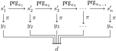
For completeness, we first consider a naive algorithm, illustrated in Figure 1. We expect that this algorithm will only be practical for short sequences as it requires testing the consistency of constraint sets involving too many variables.

Similarly as in the single decision case, the idea of the algorithm is to build a single set of constraints which is consistent iff a specified partial state does not explain a specified sequence of decisions a1, . . . , an. Given an initial state s11 , we define the set of constraints Ca1,...,an which computes the states s11 a1 ��s12 a2 ��. . . an�1 ����s1n reached by applying the successive actions as well as the policy decisions yi � πps1i q in each of these states; we then compare the yis with the ai:

Finally, we add the constraints that s11 should complete z and that d should be false. The resulting set of constraints,

'

is consistent iff there exists a state s11 that completes z for which π generates a different sequence of decisions than the specified one; i.e., z does not explain a1, . . . , an. As before, starting with z � s1, one can then greedily try to remove propositions to compute a minimal explanation.

However in this set of constraints, the variables include n duplicates of the set of state variables X, which are needed to represent the successive states s11 . . . s1n , as well as the much larger set of variables required to represent n duplicates of the computation of π (via the constraints Cπ mentioned above). As shown in our experiments in Section 6, this makes testing consistency impractical beyond short sequences.

4.2 Forward Decomposition

We now show that it is possible to decompose the explanation so that it is easier to compute a single minimal explanation. This decomposition leads to an algorithm that need only solve a number of single decision explanation problems that is in the worst case linear in the length of the sequence. In the following, � is the function composition.

Theorem 1. Let π be a policy, s be a state, and let τ n π psq � s1 a1 �� . . . an ��� sn�1 be the n-long trajectory induced by π from s. Let z � s be a partial state and let z1, . . . , zn be a sequence of partial states defined by zi�1 � prgai � � � � � prga1 pzq. Then z explains πn psq iff for all steps i, zi explains ai in si.

The proof of Theorem 1 is in Appendix A. Theorem 1 gives us a clear procedure to verify whether a partial state z is an explanation, which is to compute the partial states zi resulting from applying the actions from z (note: zi�1 � prgai pziq) and to verify whether each zi explains ai.

Algorithm 1 Computing a minimal explanation for a sequence of decisions.

1: procedure MINIMALEXPLANATION(I, π, n, s) 2: s1 a1 �� . . . an ��� sn�1 � τ n π psq 3: z1 :� s 4: for i P t1, . . . , n � 1u do 5: zi�1 :� prgai pziq 6: for x P X do 7: explains :� True 8: for i P t1, . . . , nu do � Testing condition of Th. 1 9: zi :� zi �x 10: if pzi explains aiq then � Eq. 1 11: explains :� False 12: break 13: if x P Xeffpaiq then 14: break � Can stop now (cf. Eq. 2) 15: if explains then �Must reinsert x 16: for j P t1, . . . , iu do zj :� zj ' px � sjrxsq 17: return z1

In the algorithm that we propose next, we use the additional property: for any variable x, prgai � � � � � prga1 pz � xq �

(2)

The first case is useful because it means prgai �� � ��prga1 pz� xq explains ai�1 iff prgai � � � � � prga1 pzq does; so as soon as variable x appears in the effects of ai, we will be able to ignore the condition of Theorem 1 that zk should explain ak in sk for all k ¡ i. The second case is useful because it makes it easy to compute prgai � � � � � prga1 pz � xq from prgai � � � � � prga1 pzq.

Our procedure is described in Algorithm 1. In Lines 3-5, the algorithm initialises the variables zi, mirroring the variables from Theorem 1 for explanation z :� s. Line 6 starts the loop in which each variable x is tentatively removed from the explanation. The variable explains will record whether z � x explains the sequence; until proven otherwise, it is assumed it does. The inner loop from Line 8 verifies the condition of Theorem 1. After zi is updated (using the second case of Eq. 2), the consistency check (Eq. 1) is performed on Line 10. If zi does not explain action ai, the inner loop is stopped; the loop from Line 16 will then undo the update. Otherwise, the inner loop moves to the next step i � 1 except if variable x is mentioned in the effects of ai in which case the loop can be stopped (first case of Eq. 2).

This algorithm requires Opn �mq calls to the consistency solver where n is the length of the sequence of m is the number of state variables.

We illustrate this algorithm with our running example. We assume Yvette uses the policy described in Figure 2. We note that this policy recommends sub-optimal actions (e.g., driving to the ATM and then purchasing a pass online when it is raining), which our approach can also handle. The initial state, and so the initial explanation, is z � tFriday, Sunny, NoCash, NoPass, AtHome, . . . u.

1. If has passed the TollGate, has a pass, or has some cash, drive towards the destination.
2. Otherwise, if not at the ATM, drive towards the ATM.
3. Otherwise, if it is sunny, withdraw cash.
4. Otherwise, purchase a pass online.

Figure 2: The policy given to Yvette (without goal action ag)

Algorithm 1 starts by removing Friday from the explanation, leading to z1 � z11 � zatFridayu. We find that it is impossible to instantiate the only free variable (day of the week) in such a way that a decision different from DriveToATM is taken; in other words, z11 explains the first decision. Progressing z11 gives us z12 � tSunny, NoCash, NoPass, AtATM, . . . u. This partial state also explains the second decision (WithdrawCash), and so on until the end of the sequence. Therefore, z1 explains the whole sequence.

Then, Algorithm 1 removes Sunny from the explanation. The partial state is therefore z2 � z21 � z1 a tSunnyu. Partial state z2 explains the first decision (DriveToATM). Progressing z21 gives us z22 � tNoCash, NoPass, AtATM, . . . u. This time, we find that a state in which Yvette is at the ATM and the weather is rainy will yield a different decision (PurchasePass) than the second decision (WithdrawCash). Therefore, z2 does not explain the sequence and Sunny is added back to the explanation. Similarly, the algorithm would then try and fail to remove the subsequent propositions.

5 Implementation

We use Algorithm 1 to explain the recommendations of ASNet policies [Toyer et al., 2018] for classical planning domains. This requires implementing the consistency test on line 10 of the algorithm for ASNets, which have a complex structure and nonlinear activation functions. Our encoding, presented below, is supported by mixed integer programming (MIP) solvers such as Gurobi [Gurobi Optimization, LLC, 2023], and builds on the principles underlying the MIP encodings of simpler networks used in verification or single-decision explanations (see e.g. [Fischetti and Jo, 2018]). Clearly the framework presented in the previous section is general enough to apply to any policy representation for which the consistency test can be implemented. We chose ASNets as they can learn sparse policies which are easier to scrutinise for testing purposes, and make the consistency test computationally feasible, at least for small problems.

5.1 ASNets

ASNets are neural networks dedicated to planning, trained to produce policies that apply to any problem instance from a given planning domain modelled in (P)PDDL [Younes and Littman, 2004]. An ASNet consists of L alternating action and proposition layers, beginning and ending with an action layer. In each action layer (resp. proposition layer), each action (resp. proposition) of the planning instance is represented by an action module (resp. proposition module). Modules in one layer are connected to related modules in the next layer, where a proposition p and action a are related, written Rpa, pq iff p appears in the precondition or effect of a. This enables relevant information to be efficiently propagated.

An ASNet is capable of learning policies that generalise to problem instances of different size from the same domain thanks to a weight sharing mechanism whereby the action (resp. proposition) modules from the same layer that are ground instances of the same action schema (resp. the same predicate), have the same weights. Here we omit details such as the use of skip connections and the more complex definition of relatedness in [Toyer et al., 2020], but our implementation supports them.

Action Layers. At layer l, excluding the first and last layer, the module for action a takes as input a vector ula which is constructed by enumerating the propositions p1, . . . , pM related to a, and concatenating the outputs ψl�1 p1 , . . . , ψl�1 pM of these propositions' modules from the previous layer. That is ula � rψl�1 p1 . . . ψl�1 pM sT . The output of the module is the vector φla � fpW laula � bla q where W la is a weight matrix, bla a bias vector, and f a nonlinearity. ASNets use exponential linear units (ELU), i.e. fpxq � x if x ¥ 0 and ex �1 otherwise. Note that except for the final layer, the output vectors of all modules in the network have the same dimension d.

Proposition Layers. At layer l, the module for proposition p takes as input a vector vlp constructed by enumerating the actions that are related to the proposition, pooling from the outputs of their modules at layer l if they share the same action schema, and concatenating the results. That is vlp � rpoolptφla | oppaq � o1 ^ Rpa, pquq . . . poolptφla | oppaq � oS ^ Rpa, pquqsT , where pool represents maxpooling and oppaq is the action schema of action a. Similarly as for action modules, the output of the proposition module is the vector ψlp � fpW lp vlp � blp q.

First Layer. The input to an action module of the first layer are the boolean values (0 or 1) of all its related propositions p1, . . . , pM in the current state s, booleans indicating whether each of these propositions is true in the goal, and a boolean indicating whether the action is applicable in s. That is the input vector is u1a � rσ γ ϵsT , where σ P t0, 1uM with σj � 1 iff pj P s, γ P t0, 1uM with γj � 1 iff pj P g, and ϵ � 1 iff a P Apsq.

Last Layer. The output of an action module in the final layer l � L is a single logit φLa representing the unnormalised probability that this action should be taken in the current state s given as input to the network. When, as in this paper, a deterministic policy is sought, the applicable action a P Apsq with maximum φLa is selected by the policy, breaking ties consistently.

5.2 MIP Encoding

The main purpose of the encoding is to answer consistency queries where only some of the inputs to the ASNet are given, and its output is constrained. The key decision variables in the MIP model fall into 3 categories: variables representing the network inputs, its outputs, and the action and proposition modules. As is well known from other MIP encodings of neural networks, one also needs auxiliary variables to encode the activation functions. Parameters include the weight matrices and bias vectors described above. The MIP has no objective function since we are only testing for consistency.

Policy Inputs. We encode each element in the input of an ASNet (current state propositions, goal proposition, applicable actions) using the following binary variables: Sp is true iff proposition p is true in the current state, Gp is true iff proposition p is true in the goal, and Ea is true iff a is applicable in the current state. Since a key feature of the MIP model is to allow specifying partial states as input, we must add constraints capturing when actions are applicable: action a is applicable when Sp � 1 for all p P prepaq.

Moreover, ASNets only support boolean propositions p � px � vq for x P X and v P Dx. To encode SAS� state variables, we add mutex constraints ensuring that at most one proposition assigning a value to a given variable can be true.

Action Modules. To encode action modules, we define the MIP variables pPACla qi representing the ith element of the pre-activation vector (omitting the non-linearity f) of the module for action a in layer l, and pOUTla qi representing the ith element of the output vector φla of this module. For an action a with related propositions p1, . . . , pM, we have, taking

Proposition Modules. Similarly, we define pPAClp qi and pOUTlp qi for each proposition p. For proposition modules we additionally need variables pPOOLlp,o qi to represent the ith element of the pooled vector over actions related to p sharing the action schema o. If related actions belong to S action schemas o1, . . . oS, we have, taking j � ps � 1qd � k

Activations. The encoding of f as the ELU function is very similar to the encoding of ReLU in MIP [Fischetti and Jo, 2018] and is the same for proposition and action modules. Given a proposition or action b we define the auxiliary variables ptlb qi and pslb qi to store the positive and negative component of the variable pPAClb qi, respectively, and pzlb qi which is an indicator variable for the sign of pPAClb qi. This leads to the following constraints (note that Gurobi linearises the exponential, see [Gurobi Optimization, LLC, 2023, p584-586])

Policy Output. The chosen action is the applicable action a maximising the output φLa of the final layer's modules. We enforce this using the following additional variables: Ca which is a binary variable true iff action a is chosen, and Vmax which is the maximal value of φLa for applicable actions.

Moreover, ties must be broken consistently to prevent the solver to select another action tied at the maximum value with the one currently tested. This issue frequently occurs when the problem has some symmetries, as e.g. in the Gripper domain where our ASNet policy often gives equal value to picking up the various balls in a room. Let Ma be a boolean variable true iff action a has maximum value, and � be the total ordering over the action set A used by the policy to break ties, we break ties by favouring the action coming earlier in the ordering.

These additional constraints greatly increase the runtime of the MIP solver. Therefore we apply them only when needed. We first run the MIP without them, and if the solver finds a solution which selects an action tied with the action tested, we re-run the MIP with the tie-breaking constraints.

Temporary Constraints. The above constraints constitute the encoding Cπ of the ASNet policy and only needs to be built once for a given sets X and A of state variables and actions. For each consistency query involving a planning instance I � xX,A, gy, an action decision a, and a candidate explanation z, it suffices to temporarily add the following constraints to set g as the goal, prevent a to be chosen by the policy, and look for a possible completion s of z.

6 Experimental Results

The goal of our experiments is to evaluate how effective abductive explanations are in explaining why a policy recommends a particular course of actions. In particular, we consider what fraction of the input appears in the minimal explanation: the smaller the explanation, the easier it is for a human to interpret. We also focus on the scalability of Algorithm 1 as the size of the policy increases, taking that of the naive algorithm in Section 4.1 as a baseline. Finally, we evaluate the sensitivity of the explanation size and runtime to the ordering in which variables are processed by our algorithm. For reproducibility, our repository https://github.com/ReneeSelvey/policy-explanations provides our algorithm implementation, benchmarks used, learnt policies, and the scripts to learn them and run the experiments.

6.1 Experimental Setup

Hardware. All experiments were run on a machine with an AMD Ryzen Threadripper 3990X CPU, with 64 cores/128 threads, a clock speed of 2.9 GHz base, 4.3 GHz max boost, and 128 GB of memory of which we used 64 GB.

MIPConfiguration. Gurobi version 9.1.2 is theMIP solver used for the experiments. To ensure the model is accurate enough for our experiments, we set the integer feasibility tolerance (IntFeasTol) to 10�9 and the error for function approximations (FuncPieceError) to 10�6 .

ASNet policies. We took all deterministic domains and training instances from the code distributions of [Toyer et al., 2020] and [Steinmetz et al., 2022]. We ran the script provided by Toyer using 1 core, an 8h timeout, and 64 GB of memory to learn, from these instances, two-layer (i.e. two proposition layers and three action layers) sparse policies with skip connections and without heuristic inputs. As described in [Toyer et al., 2020, Sec. 6], the ℓ1-regulariser used to train sparse policies results in many modules having coefficient so close to zero that they are insignificant to the output of the network and are prunned by the ASNet sparsification procedure. Hence, these modules do not appear in the MIP model, making a simpler model to solve.

6.2 Domains and Problems

We kept the domains for which the learnt policy could solve any problem within 150 execution steps, amongst a test set of 20 randomly generated small problems for that domain. This resulted in 4 policies for the domains of Blocksworld, Gripper, n-Puzzle, and Parking, which are present in the ASNets code distribution. In order to evaluate our approach, we randomly generated, for each of these domains, the set of problems described below. Explanations were only computed for problems where the policy was able to reach the goal within 150 steps. Each explanation problem was run with a time limit of 3h, except for Gripper for which the timeout was 4h.

Blocksworld. Experiments were conducted on 10 problems of each size (2-10 blocks) for a total of 90 problems. The policy was able to solve 71% of problems, all of which had explanations computed within the time limit.

Gripper. Explanationswere computed using problemswith 2 rooms and 1-15 balls. The policy was able to solve all problems, and explanations could be computed for 93%.

n-Puzzle. Experiments were conducted on all solvable and non-trivial combinations of 3-puzzle problems (on a 2x2 grid). Out of these 11 problems, the policy was correctly able to solve all instances and our approach could compute all explanations.

Parking. Problems in the parking domain comprised of 2 cars and 2-4 curbs. Out of the 22 total problems, the policy reached the goal for 55% and we were able to compute explanations for all of these within the time limit.

To avoid numerical instability issues, we excluded from our results below any problem for which a MIP call exceeded a constraint violation tolerance of 5e-01. This led to 8 Blocksworld and 2 Parking problems being excluded. Note moreover that we would have liked to evaluate our algorithm on larger n-Puzzle or Parking instances. However, we couldn't learn sparse policies capable of solving such instances, and the non-sparse (standard) ASNet policies produced with the ℓ2-regulariser were too large for the MIP solver.

6.3 Results

Size of Explanations

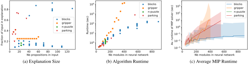
Figure 3a shows the size of the explanation obtained as a fraction of the size of the input. In all domains, Algorithm 1 produces an explanation smaller than ASNet's input. For nPuzzle, the small explanations are due to many static propositions. The grid in the problem is defined as propositions listing the neighbours of each position. As this grid is static, this will not appear in the explanation.

Many Blocksworld's explanations are also particularly small as many propositions remain false along the plan execution and are irrelevant, and some of the true propositions can be deduced from a small set of others. For instance, consider the optimal plan for a 3 block problem with b2 on b1 on b3 initially and b3 on b2 and b1 on the table in the goal. The explanation clearpb2q, onpb2, b1q, ontablepb1q returned by Algorithm 1 suffices to make the plan applicable and does not need to mention b3 which is obviously on the table.

The bulk of Gripper's explanations (i.e. all except for n � 1, 2, 14 balls) are steady at 1/4 of the input propositions. These explanations are obtained when the algorithm makes the best choices about which propositions to remove. They mention the actual location of the balls and Robby. The other propositions representing locations can be deduced to be false, and at that point the status of the grippers become irrelevant.

Scalability

Most of the runtime is spent in MIP consistency tests. As can be seen from the size of problems we can address, reasoning about neural networks using MIP is a serious bottleneck. Across all domains, we have observed that, as input propositions progressively get removed from the explanation, consistency tests generally become harder. This is because proving inconsistency generally becomes harder, and whilst proving consistency becomes easier, it leads us to reinsert the proposition, so the algorithm never reaches the easy region of the consistent side of the phase boundary. This behaviour is common with optimisation problems.

There are differences in scalability amongst the domains however. Figure 3b shows the runtime of the algorithm as a function of the size of the neural network policy for the problem. Gripper scaled the worst as a function of the number of modules in the network. This is due to two main factors. Firstly gripper plans are longer than those recommended by the policies for the other domains (from length 3 for n � 1 to 41 for n � 14) and therefore lead to a large number of MIP calls (from 16 to 1442). Secondly, and more importantly, the average runtime of MIP calls (shown in Figure 3c) is also larger than for the other domains, due to a large amount of tie-breaking being necessary for many problems. For n � 1 to 9, only the odd numbered problems required tie-breaking as is visible on both Figures 3b and 3c.

Blocksworld scaled the best. It has reasonably long plans (2 to 26 actions), and leads to even more MIP calls than Gripper (17 to 2176) because propositions survive longer through the inner loop before being reinstated in the explanation or definitely ruled out. However, as shown in Figure 3c, the MIP problems are relatively easy to solve, in part because, except for two problems, almost no tie-breaking was necessary.

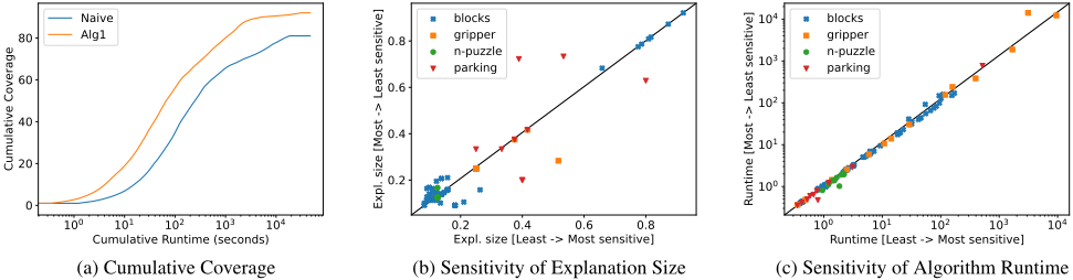
We implemented the naive approach as a baseline for scalability comparison. The naive algorithm can solve the Parking and n-Puzzle problems as these have short plans (1 to 6 actions). It could not solve Gripper problems after n � 4 nor the largest Blocksworld problems. Moreover, as shown in Figure 4a, it is 5 to 10 times slower than Algorithm 1 on our benchmark problems.

Sensitivity to Removal Ordering

As explained in Section 3, there are potentially many minimal explanations for a policy trajectory. The explanation obtained, as well as its size and the runtime of Algorithm 1, depend on the order in which input variables are selected for removal on line 6 of the algorithm. In order to provide an idea of how stable the minimal explanation size and runtime are to the ordering, we use a heuristic inspired by [Wu et al., 2022; Vinzent et al., 2023], which computes the sensitivity of the network output to changes of value to each input variable. We then compare the explanations obtained by removing variables in increasing and decreasing order of their sensitivity, respectively. We measure variable sensitivity as follows.

where, by slight abuse of notation, πpa, sq is the (unnormalised) probability of the policy predicting action a in state s, before determinisation (this corresponds to the value of OUTLa in our MIP encoding). Hence, for each state in the trajectory, we take the difference between the output of the neural network for the action prescribed, and that of the best other action that would be prescribed if we changed the value of the variable x. The variable sensitivity senpxq is the minimum of this difference over the states in the trajectory.

Figures 4b and 4c compare the explanation size and algorithm runtime, respectively, obtained under the two removal orderings. These figures suggest that except for Parking, the runtime and explanation size are only very moderately sensitive to the ordering.

7 Conclusion, Limits, and FutureWork

We have extended abductive explanations to sequences of decisions recommended by neural network policies. Our decomposition approach to find a single minimal explanation incurs no overhead in comparison with the single decision case, once the length of the sequence is factored in.

Our approach makes a number of limiting assumptions which we discuss here together with possible extensions and future work. The first assumption is the availability of a symbolic planning model. An interesting avenue for future work is the extension of this approach to learnt planning models, also represented as neural networks.

We also assumed that actions have simple, unconditional effects. Conditional effects can be handled by our naive algorithm. However, Theorem 1 does not allow for them because it is impossible to apply conditional effects to a partial state. We assumed that we have no background knowledge, i.e. constraints that restrict the set of possible states [Thi´ebaux et al., 2005; Rintanen, 2017]. These can greatly simplify explanations. Yu et al. [2023] showed that in the single decision case, adding the background knowledge K as another conjunct to the consistency tests performed by the greedy algorithm preserves the minimality of explanations. This property carries over to the multiple decision case and our naive algorithm. However, our decomposition algorithm may not return a minimal explanation with this augmented consistency test, because the set of reachable states cannot be represented by intersections of partial states with K. We leave an efficient treatment of conditional effects and background knowledge for future work.

We have assumed that the actions and the policy are deterministic. Handling stochastic actions and/or policies could be achieved by generating explanations that pertain to a finite tree of actions reachable with non-zero probability from the initial state. This would require applying progression and consistency tests at each branch of the tree. Handling stochastic policies would additionally require a more complex consistency test, as the decision d becomes a probability distribution over actions and the test must establish that it is not possible for the policy to return a different distribution.

Another avenue for future work is the generation of all (set-inclusion) minimal explanations and of minimum cardinality explanations. This is likely to require a different decomposition of the problem than the one presented here, as well as effective heuristics to guide search. Finally, even in the single decision case, methods for computing formal explanations of neural networks suffer from scalability issues due to the expensive consistency test. New breakthroughs in MIP and SMT methods for analysing neural networks, new problem abstractions, and approximate explanation methods will be needed for these approaches to flourish.

A Proof of Theorem 1

Lemma 1. If z explains a1, . . . , an, then for all i P t0, . . . , n� 1u, zi�1 :� prgai � � � � � prga1 pzq explains ai�1.

We shall prove that for all i P t0, . . . , n � 1u, for all state si�1 that completes zi�1, there exists si such that i) ai is applicable in si, ii) si ai �� si�1 is a transition of the planning domain, and iii) si completes zi. By recursion, we end up with a state s1 that completes z1 such that s1 a1 �� s2 a2 �� . . . ai �� si�1. Since s1 completes z1 � z, we know that πn ps1q � a1, . . . , an. Therefore, πpsi�1q � ai�1. As this is true for all si�1, zi�1 explains ai�1.

The proof will be done by induction, i.e., we assume that it is true for i. (Base case for i � 0 is trivially true as z1 � z.) Given state si�1, we choose si as one of the states satisfying

We prove that si satisfies the three points above.

i) Eq. 3 clearly enforces the precondition prepaiq, so ai is indeed applicable in si.

ii) We note

which can be simplified by

We also note that all variables x P X are specified in prgai psiq, regardless of the choice of si. Consider any variable x; we show that prgai psiqrxs � si�1rxs holds by looking at 3 cases:

• If x P Xeffpaiq , then prgai psiqrxs � effai pxq and, since zi�1 � prgai pziq, si�1rxs � zi�1rxs � effai pxq.
• If x P XprepaiqzXeffpaiq , then prgai psiqrxs � sipxq � prepaiqrxs since ai is applicable in si. Furthermore, we note that si�1 completes prga1 pziq and that zirxs � prepaiqrxs since (by induction) zi explains ai; therefore si�1rxs � prepaiqrxs � prgai psiqrxs.

iii) Does si complete zi? Since, by construction, si completes zi ' ppsi�1 a effpaiqq ' prepaiqq, the question is whether some assignment in the right operand of zi ' contradicts an assignment in si. We know that zi explains ai, so preai will not contradict zi. State si�1 completes zi�1 which differs with zi only on effpaiq. However, the expression above removes effpaiq from si�1, so that the right operand does not map any variable to a different value than zi.

Lemma 2. Let z be a partial state, and for all i P t0, . . . , n� 1u, zi�1 :� prgai � � � � � prga1 pzq. If for all i, zi explains ai, then z explains a1, . . . , an.

Assume that zi explains ai for all i. Let s be a state completing z and let s1 a1 �� . . . an ��� sn be the trajectory obtained by applying the sequence of actions a1, . . . , an from s1 � s. We shall prove πpsiq � ai for all i (which proves that π recommends a1, . . . , an); this is proven by showing that si completes zi.

The state si�1 is defined as prgai � � � � � prga1 psq. Do we have @x P Xzi�1 . si�1rxs � zi�1rxs? Let j be the largest index in t1, . . . , iu such that x P Xeffpajq . If j does not exist, then si�1rxs � srxs � zrxs � zi�1rxs. Otherwise, si�1rxs � effpajqrxs � zi�1rxs. Either way, the variables of si�1 map to the same value as those of zi�1. Therefore, zi�1 explains ai�1 in si�1.

Theorem 1 is a consequence of Lemmas 1 and Lemma 2.

Acknowledgements

We thank the anonymous reviewers for their useful comments which helped to improve the paper. This work has received funding from the European Union's Horizon Europe Research and Innovation program under the grant agreement TUPLES No 101070149. S. Thi´ebaux was also supported by ARC grant DP220103815. A. Grastien and S. Thi´ebaux are members of the Humanising Machine Intelligence project at ANU.