Stochastic Population Update Can Provably Be Helpful in Multi-Objective Evolutionary Algorithms

1 Introduction

Multi-objective optimization refers to an optimization scenario that there are more than one objective to be considered at the same time, which often appears in real-world applications. Since the objectives of a multi-objective optimization problem (MOP) are usually conflicting, there does not exist a single optimal solution, but instead a set of solutions which represent different trade-offs between these objectives, called Pareto optimal solutions. The images of all Pareto optimal solutions of an MOP in the objective space are called the Pareto front. In multi-objective optimization, the goal of an optimizer is to find a good approximation of the Pareto front.

∗This work was supported by the National Science Foundation of China (62022039, 62276124). Chao Qian is the corresponding author.

Evolutionary algorithms (EAs) [B¨ack, 1996; Eiben and Smith, 2015] are a large class of randomized heuristic optimization algorithms, inspired by natural evolution. They maintain a set of solutions, i.e., a population, and iteratively improve it by generating new solutions and selecting better ones. Due to the population-based nature, EAs are wellsuited to solving MOPs, and have been widely used in various real-world scenarios [Coello Coello and Lamont, 2004; Deb, 2011; Zhou et al., 2019].

In multi-objective EAs (MOEAs), two key components are solution generation and population update. The former is concerned with parent selection and reproduction (e.g., crossover and mutation), while the latter (also called environmental selection or population maintenance) is concerned with maintaining a solution set which represents the best solutions found so far. In the area of evolutionary multi-objective optimization, the research focus is mainly on population update. That is, when designing an MOEA, attention is placed on how to update the population by newly-generated solutions so that a set of well distributed non-dominated solutions is preserved. With this aim, many selection criteria emerge, such as non-dominated sorting [Goldberg, 1989], crowding distance [Deb et al., 2002], scalarizing functions [Zhang and Li, 2007] and quality indicators [Zitzler and K¨unzli, 2004].

A prominent feature in population update of MOEAs is its deterministic manner (apart from random tie breaking). That is, the next-generation population is formed by always selecting the first population-size ranked solutions out of the collections of the current population and newly-generated solutions. It is believed that a population formed by the best solutions has a higher chance to generate even better solutions.

In this paper, we challenge this belief. We analytically show that introducing randomness into the population update procedure may be beneficial for the search. Specifically, we consider a well-established MOEA, S metric selection evolutionary multi-objective optimization algorithm (SMSEMOA) [Beume et al., 2007], and propose a simple stochastic population update method. Instead of removing the worst solution 1 from the collections of the current population and newly-generated solution, the proposed stochastic method first randomly selects a subset from the collections and then removes the worst solution from the subset. We theoretically show that this simple modification makes SMS-EMOA significantly better on OneJumpZeroJump, a bi-objective optimization problem commonly used in theoretical analyses of MOEAs [Doerr and Zheng, 2021; Doerr and Qu, 2022a; Doerr and Qu, 2022b; Doerr and Qu, 2022c]. More specifically, we first prove that the expected running time of the original SMS-EMOA is O(µnk ) and Ω(nk ), where µ is the population size, n is the problem size and k (2 ≤ k < n/2) is the parameter of the problem. Then, we prove that using stochastic population update can decrease the expected running time to O(µnk · min{1, µ/2k/4 }). In other words, stochastic population update can bring an exponential acceleration when µ = poly(n) and k = Ω(n), where poly(n) denotes any polynomial of n. The intuitive reason for this occurrence is that by introducing randomness into the population update procedure, the evolutionary search can go across inferior regions between different Pareto optimal solutions more easily, thus facilitating to find the whole Pareto front. Experiments are also conducted to verify our theoretical results.

1 SMS-EMOA adopts a (µ + 1) steady state mode, where selecting the µ best solutions means removing the worst solution.

There is an increasing interest to study MOEAs theoretically. Primitive theoretical work mainly focuses on analyzing the expected running time of GSEMO/SEMO, a simple MOEA which employs the bit-wise/one-bit mutation operator to generate an offspring solution in each iteration and keeps the non-dominated solutions generated-so-far in the population, in solving multi-objective synthetic and combinatorial optimization problems [Giel, 2003; Laumanns et al., 2004a; Laumanns et al., 2004b; Neumann, 2007; Horoba, 2009; Giel and Lehre, 2010; Neumann and Theile, 2010; Doerr et al., 2013; Qian et al., 2013; Bian et al., 2018]. Based on (G)SEMO, the effectiveness of some parent selection and reproduction methods, e.g., greedy parent selection [Laumanns et al., 2004b], diversity-based parent selection [Friedrich et al., 2010; Covantes Osuna et al., 2020], fairness-based parent selection [Laumanns et al., 2004b; Friedrich et al., 2011], fast mutation and stagnation detection [Doerr and Zheng, 2021], crossover [Qian et al., 2013], and selection hyperheuristics [Qian et al., 2016], has also been studied.

Recently, researchers have started attempts to analyze practical MOEAs. The expected running time of (µ + 1) SIBEA, i.e., a simple MOEA using the hypervolume indicator to update the population, was analyzed on several synthetic problems [Brockhoff et al., 2008; Nguyen et al., 2015; Doerr et al., 2016], which contributes to the theoretical understanding of indicator-based MOEAs. Later, people have started to consider well-established algorithms in the evolutionary multi-objective optimisation area. For example, Huang et al. [2021] considered MOEA/D, and examined the effectiveness of different decomposition methods by comparing the running time for solving many-objective synthetic problems. Very recently, Zheng et al. [2022] analyzed the expected running time of NSGA-II (which uses non-dominated sorting and crowding distance mechanisms to update the population) for solving OneMinMax and LOTZ. Later on, Zheng and Doerr [2022] considered a modified crowding distance method, which updates the crowding distance of solutions once the solution with the smallest crowding distance is removed, and proved that the modified method can approximate the Pareto front better than the original crowding distance method in NSGA-II. Bian and Qian [2022] proposed a new parent selection method, stochastic tournament selection (i.e., k tournament selection where k is uniformly sampled at random), to replace the binary tournament selection of NSGA-II, and proved that the method can decrease the expected running time asymptotically. There is also some work analyzing the effectiveness of the mutation [Doerr and Qu, 2022a] and crossover [Doerr and Qu, 2022c; Dang et al., 2023] operators in NSGA-II. The lower bounds of NSGA-II solving OneMinMax and OneJumpZeroJump have also been analyzed [Doerr and Qu, 2022b].

Our running time analysis about SMS-EMOA contributes to the theoretical understanding of another major type of MOEAs, i.e., combining non-dominated sorting and quality indicators to update the population, for the first time. More importantly, our work presents a potential drawback of an important component, i.e., population update, in existing MOEAs. That is, instead of updating the population in a deterministic way, introducing randomness may be helpful for the search, even reducing the expected running time of MOEAs exponentially. Though being proved in a special case, this finding may hold more generally, and may inspire the design of more efficient MOEAs in practice.

2 Preliminaries

In this section, we first introduce multi-objective optimization and SMS-EMOA, and then present a new population update method, i.e., stochastic population update. Finally, we introduce the OneJumpZeroJump problem studied in this paper.

2.1 Multi-objective Optimization

Multi-objective optimization aims to optimize two or more objective functions simultaneously, as shown in Definition 1. Note that in this paper, we consider maximization (minimization can be defined similarly), and pseudo-Boolean functions, i.e., the solution space X = {0, 1}n . The objectives are usually conflicting, thus there is no canonical complete order in the solution space X , and we use the domination relationship in Definition 2 to compare solutions. A solution is Pareto optimal if there is no other solution in X that dominates it, and the set of objective vectors of all the Pareto optimal solutions constitutes the Pareto front. The goal of multi-objective optimization is to find the Pareto front or its good approximation.

Definition 1 (Multi-objective Optimization). Given a feasible solution space X and objective functions f1, f2, . . . , fm, multi-objective optimization can be formulated as

Definition 2 (Domination). Let f = (f1, f2, . . . , fm) : X → Rm be the objective vector. For two solutions x and y ∈ X :

• x weakly dominates y (denoted as x ⪰ y) if for any 1 ≤ i ≤ m, fi(x) ≥ fi(y);
• x dominates y (denoted as x ≻ y) if x ⪰ y and fi(x) > fi(y) for some i;
• x and y are incomparable if neither x ⪰ y nor y ⪰ x.

Algorithm 1 SMS-EMOA

Input: objective functions f1, f2 . . . , fm, population size µ Output: µ solutions from {0, 1}n

• 1: P ← µ solutions uniformly and randomly selected from {0,1}n with replacement;
• 2: while criterion is not met do
• 3: select a solution x from P uniformly at random;
• 4: generate x′ by flipping each bit of x independently with probability 1/n;
• 5: P ← POPULATION UPDATE (P ∪ {x′ })
• 6: end while
• 7: return P

Algorithm 2 POPULATION UPDATE (Q)

Input: a set Q of solutions, and a reference point r ∈ Rm Output: |Q|-1 solutions fromQ

• 1: partition Q into non-dominated sets R1,R2, . . . ,Rv;
• 2: let z = argminx∈Rv ∆r(x,Rv);
• 3: return Q\ {z}

2.2 SMS-EMOA

The SMS-EMOA algorithm [Beume et al., 2007] as presented in Algorithm 1 is a popular MOEA, which employs nondominated sorting and hypervolume indicator to evaluate the quality of a solution and update the population. SMS-EMOA starts from an initial population of µ solutions (line 1). In each generation, it randomly selects a solution from the current population (line 3), and then applies bit-wise mutation to generate an offspring solution (line 4). Then, the worst solution in the union of the current population P and the newly generated solution is removed (line 5), by using the POPULATION UPDATE subroutine as presented in Algorithm 2.

As can be seen in Algorithm 2, the POPULATION UPDATE subroutine first partitions a set Q of solutions (where Q = P ∪ {x′ } in Algorithm 1) into non-dominated sets R1,R2, . . . ,Rv (line 1), where R1 contains all the nondominated solutions in Q, and Ri (i ≥ 2) contains all the non-dominated solutions in Q \ ∪i-1 j=1Rj. Then, one solution z ∈ Rv that minimizes ∆r(x,Rv) := HVr(Rv) - HVr(Rv \ {x}) is removed (lines 2-3), where HVr(Rv) = Λ( ∪x∈Rv {f ′ ∈ Rm | ∀1 ≤ i ≤ m : ri ≤ f ′ i ≤ fi(x)}) denotes the hypervolume of Rv with respect to a reference point r ∈ Rm (satisfying ∀1 ≤ i ≤ m, ri ≤ minx∈X fi(x)), and Λ denotes the Lebesgue measure. The hypervolume of a solution set measures the volume of the objective space between the reference point and the objective vectors of the solution set, and a larger hypervolume value implies a better approximation ability with regards to both convergence and diversity. This implies that the solution with the least value of ∆ in the last non-dominated set Rv can be regarded as the worst solution in Q, which is thus removed.

2.3 Stochastic Population Update

Previous MOEAs only considered deterministic and greedy population update methods, i.e., a dominating solution or a solution with better indicator value is always preferred. How-

Algorithm 3 STOCHASTIC POPULATION UPDATE (Q)

Input: a set Q of solutions, and a reference point r ∈ Rm Output: |Q|-1 solutions fromQ

• 1: Q′ ← ⌊|Q|/2⌋ solutions uniformly and randomly selected fromQwithout replacement;
• 2: partition Q′ into non-dominated sets R1,R2, . . . ,Rv;
• 3: let z = argminx∈Rv ∆r(x,Rv);
• 4: return Q\ {z}

ever, these methods may be too greedy, and thus limit the performance of MOEAs. In this paper, we introduce STOCHASTIC POPULATION UPDATE as presented in Algorithm 3 into SMS-MOEA, to replace the original POPULATION UPDATE procedure in line 5 of Algorithm 1. These two procedures are similar, except that the removed solution is selected from a subset Q′ of Q in Algorithm 3, instead of from the entire set Q, where Q′ consists of N solutions chosen randomly from Q. Note that we set N = ⌊|Q|/2⌋ here for examination, while other values of N can also be used in practical applications.

2.4 OneJumpZeroJump Problem

The OneJumpZeroJump problem is a multi-objective counterpart of the Jump problem, a classical single-objective pseudo-Boolean benchmark problem in EAs' theoretical analyses [Doerr and Neumann, 2020]. The goal of the Jump problem is to maximize the number of 1-bits of a solution, except for a valley around 1n (the solution with all 1-bits) where the number of 1-bits should be minimized. Formally, it aims to find an n-bits binary string which maximizes

where k ∈ [2..n-1], and |x|1 denotes the number of 1-bits in x. Note that we use [a..b] (where a, b ∈ N, a ≤ b) to denote the set {a, a + 1, . . . , b} of integers throughout the paper.

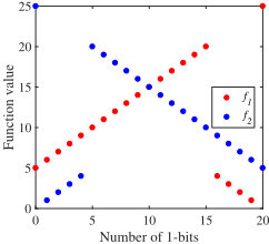
The OneJumpZeroJump problem as presented in Definition 3 is constructed based on the Jump problem, and has been widely used in MOEAs' theoretical analyses [Doerr and Zheng, 2021; Doerr and Qu, 2022a; Doerr and Qu, 2022b; Doerr and Qu, 2022c]. Its first objective is the same as the Jump problem, while the second objective is isomorphic to the first one, with the roles of 1-bits and 0-bits exchanged. Figure 1 illustrates the values of f1 and f2 with respect to the number of 1-bits of a solution.

Definition 3. [Doerr and Zheng, 2021] The OneJumpZeroJump problem is to find n bits binary strings which maximize

where k ∈ Z ∧ 2 ≤ k < n/2, and |x|1 and |x|0 denote the number of 1-bits and 0-bits in x, respectively.

According to Theorem 5 of [Doerr and Zheng, 2021], the Pareto set of the OneJumpZeroJump problem is

and the Pareto front is

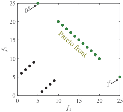
whose size is n - 2k + 3. Figure 2 illustrates the objective vectors and the Pareto front. We use

and

to denote the inner part of the Pareto set and Pareto front, respectively. Note that each objective value of the OneJumpZeroJump problem must be larger than zero, thus we set the reference point r = (0, 0) in SMS-EMOA.

3 Running Time Analysis of SMS-EMOA

In this section, we analyze the expected running time of SMSEMOA in Algorithm 1 for solving the OneJumpZeroJump problem. Note that the running time of EAs is often measured by the number of fitness evaluations, the most timeconsuming step in the evolutionary process. As SMS-EMOA generates only one offspring solution in each generation, its running time is just equal to the number of generations. We prove in Theorems 1 and 2 that the upper and lower bounds on the expected number of generations of SMS-EMOA solving OneJumpZeroJump are O(µnk ) and Ω(nk ), respectively. Note that we use poly(n) to denote any polynomial of n.

Theorem 1 (Upper bound). For SMS-EMOA solving OneJumpZeroJump, if using a population size µ such that n - 2k + 3 ≤ µ, then the expected number of generations for finding the Pareto front is O(µnk ).

Theorem 2 (Lower bound). For SMS-EMOA solving OneJumpZeroJump with n - 2k = Θ(n), if using a population size µ such that n-2k+3 ≤ µ = poly(n), then the expected number of generations for finding the Pareto front is Ω(nk ).

The proof of Theorem 1 relies on Lemma 1, which shows that once an objective vector f ∗ in the Pareto front is found, it will always be maintained, i.e., there will always exist a solution whose objective vector is f ∗ in the population.

Lemma 1. For SMS-EMOA solving OneJumpZeroJump, if using a population size µ such that n - 2k + 3 ≤ µ, then an objective vector f ∗ in the Pareto front will always be maintained once it has been found.

Proof. Suppose the objective vector (a, n + 2k - a), a ∈ [2k..n] ∪ {k, n + k}, in the Pareto front is obtained by SMSEMOA, i.e., there exists a solution x in Q (i.e., P ∪ {x′ } in line 5 of Algorithm 1) such that f(x) = (a, n + 2k - a). If at least two solutions correspond to the objective vector, then at least one of them will still be maintained in the next generation because only one solution is removed by Algorithm 2.

If only one solution (denoted as y) corresponds to the objective vector, then we have y ∈ R1 in the POPULATION UPDATE procedure because y cannot be dominated by any other solution; and ∆r(y, R1) = HVr(R1) -HVr(R1 \ {y}) > 0 because the region

cannot be covered by any objective vector in f({0, 1}n ) \ {(a, n + 2k - a)}. Then, we consider two cases.

(1) There exists one solution x in R1 such that k ≤ |x|1 ≤ n - k. Then, R1 cannot contain solutions whose number of 1-bits are in [1..k - 1] ∪ [n - k + 1..n - 1], because these solutions must be dominated by x. If at least two solutions in Q have the same objective vector, then they must have a zero ∆ value, because removing one of them will not decrease the hypervolume covered. Thus, for each objective vector (b, n+2k -b), b ∈ [2k..n] ∪{k, n+k}, at most one solution can have a ∆ value larger than zero, implying that there exist at most n - 2k + 3 ≤ µ solutions in R1 with ∆ > 0.

(2) Any solution x in R1 satisfies |x|1 < k or |x|1 > n - k. Note that for the solutions with the number of 1-bits in [1..k - 1], a solution with more 1-bits must dominate a solution with less 1-bits. Meanwhile, two solutions with the same number of 1-bits will have a zero ∆ value, thus R1 can only contain at most one solution in {x | |x|1 ∈ [1..k - 1]} with ∆ value larger than zero. Similarly, at most one solution in {x | |x|1 ∈ [n-k+1..n-1]} with∆value larger than zero belongs to R1. For solutions with number of 1-bits in {0, n} (note that there may exist reduplicative solutions in Q), it is also straightforward to see that at most two of them can have a ∆ value larger than zero. By the problem setting k < n/2, we have µ ≥ n - 2k + 3 ≥ 4, thus there exist at most µ solutions in R1 with ∆ value larger than zero.

Combining the above two cases, we show that there exist at most µ solutions in R1 with ∆ value larger than zero, implying that y will still be maintained in the next generation.

The main proof idea of Theorem 1 is to divide the optimization procedure into two phases, where the first phase aims at finding the inner part F ∗ I (in Eq. (2)) of the Pareto front, and the second phase aims at finding the remaining two extreme vectors in the Pareto front, i.e., F ∗ \ F ∗ I = {(k, n + k), (n + k, k)}, corresponding to the two Pareto optimal solutions 0n and 1n .

Proof of Theorem 1. We divide the optimization procedure into two phases. The first phase starts after initialization and finishes until all the objective vectors in the inner part F ∗ I of the Pareto front has been found; the second phase starts after the first phase and finishes when the whole Pareto front is found. We will show that the expected number of generations of the two phases are O(µ(n log n + kk )) and O(µnk ), respectively, leading to the theorem.

For the first phase, we consider two cases.

(1) At least one solution in the inner part S∗ I of the Pareto set exists in the initial population. Let

where H+(x) := {x′ | |x′ |1 = |x|1 + 1} and H-(x) := {x′ | |x′ |1 = |x|1 - 1} denote the Hamming neighbours of x with one more 1-bit and one less 1-bit, respectively. Intuitively, D1 denotes the set of solutions in P whose Hamming neighbour is Pareto optimal but not contained by P. Then, by selecting a solution x ∈ D1, and flipping one of the 0-bits or one of the 1-bits, a new objective vector in F ∗ I can be obtained. By Lemma 1, one solution corresponding to the new objective vector will always be maintained in the population. By repeating the above procedure, the whole set F ∗ I can be found. Note that the probability of selecting a specific solution in P is 1/µ, and the probability of flipping one of the 0-bits (or 1-bits) is (n- |x|1) · (1/n) · (1-1/n)n-1 ≥ (n|x|1)/(en) (or (|x|1/n) · (1-1/n)n-1 ≥ |x|1/(en)). Thus, the total expected number of generations for finding F ∗ I is at most ∑|x|1 i=k+1 (µen)/i + ∑n-|x|1 i=k+1 (µen)/i = O(µn log n).

(2) Any solution in the initial population has at most (k-1) 1-bits or at least (n-k+1) 1-bits. Without loss of generality, we can assume that one solution y has at most (k - 1) 1-bits. Then, selecting y and flipping (k - |y|1) 0-bits can generate a solution in S∗ I , whose probability is at least

Let g(i) = (n-i k-i)/nk-i , 0 ≤ i ≤ k - 1, then we have

implying

Thus, the expected number of generations for finding a solution in S∗ I is at most eµkk . By Lemma 1, the generated solution must be included into the population. Thus, combining the analysis for case (1), we can derive that the total expected number of generations for finding F ∗ I is O(µ(n logn+kk )).

For the second phase, we need to find the two extreme solutions1n and0n. To find 1n (or 0n ), it is sufficient to select the solution in the population P with (n - k) 1-bits (or k 1-bits) and flip its k 0-bits (or k 1-bits), whose probability is (1/µ) · (1/nk ) · (1 - 1/n)n-k ≥ 1/(eµnk ). Thus, the expected number of generations is O(eµnk ).

Combining the derived upper bounds on the expected number of generations of the two phases, the theorem holds.

The proof idea of Theorem 2 is that all the solutions in the initial population belong to the inner part S∗ I (in Eq. (1)) of the Pareto set with probability Θ(1), and then SMS-EMOA requires Ω(nk ) expected number of generations to find the two extreme Pareto optimal solutions 1n and 0n .

Proof of Theorem 2. Let G denote the event that all the solutions in the initial population belong to S∗ I , i.e., for any solution x in the initial population, k ≤ |x|1 ≤ n - k. We first show that event G happens with probability 1 - o(1). For an initial solution y, it is generated uniformly at random, i.e., each bit in y can be 1 or 0 with probability 1/2, respectively. Thus, the expected number of 1-bits in y is exactly n/2. By Hoeffding's inequality and the condition n - 2k = Θ(n) of the theorem, we have

Then, we can derive that

where the last inequality holds by Bernoulli's inequality, and the equality holds by the condition µ = poly(n).

Next we show that given event G, the expected number of generations for finding the whole Pareto front is at least nk . Starting from the initial population, if a solution x with 1 ≤ |x|1 ≤ k-1 or n-k+1 ≤ |x|1 ≤ n-1 is generated in some generation, it must be deleted because it is dominated by any of the solutions in the current population. Thus, the extreme solution 1n can only be generated by selecting a solution in S∗ I and flipping all the 0-bits, whose probability is at most 1/nk . Thus, the expected number of generations for finding 1n is at least nk .

Combining the above analyses, the expected number of generations for finding the whole Pareto front is at least (1 - o(1)) · nk = Ω(nk ).

4 Analysis of SMS-EMOAUsing Stochastic Population Update

In the previous section, we have proved that the expected number of generations of SMS-EMOA is O(µnk ) and Ω(nk ) for solving OneJumpZeroJump. Next, we will show that by employing stochastic population update in Algorithm 3, instead of the original population update procedure in Algorithm 2, SMS-EMOA can use much less time to find the whole Pareto front.

In particular, we prove in Theorem 3 that the expected number of generations of SMS-EMOA using stochastic population update is O(µnk · min{1, µ/2k/4 }) for solving the OneJumpZeroJump problem when 2(n - 2k + 4) ≤ µ. Recall from Theorem 2 that the expected number of generations of the original SMS-EMOA is Ω(nk ) when n - 2k = Θ(n) and n-2k +3 ≤ µ = poly(n). Thus, when k = Ω(n) ∧ k = n/2 - Θ(n) and 2(n - 2k + 4) ≤ µ = poly(n), using stochastic population update can bring an acceleration of at least Ω(2k/4 /µ2 ), implying an exponential acceleration. The main reason for the acceleration is that introducing randomness into the population update procedure allows a bad solution, i.e., a solution xwith |x|1 ∈ [1..k-1]∪[n-k+1..n-1], to be included into the population with some probability, thus making SMS-EMOA much easier to generate the two extreme Pareto optimal solutions 0n and 1n .

Theorem 3. For SMS-EMOA solving OneJumpZeroJump, if using stochastic population update in Algorithm 3, and a population size µ such that 2(n - 2k + 4) ≤ µ, then the expected number of generations for finding the Pareto front is O(µnk · min{1, µ/2k/4 }).

Before proving Theorem 3, we first present Lemma 2, which shows that given proper value of µ, an objective vector in the Pareto front will always be maintained once it has been found; any solution (even the worst solution) in the collections of the current population and the newly generated offspring solution can survive in the population update procedure with probability at least 1/2.

Lemma 2. For SMS-EMOA solving OneJumpZeroJump, if using stochastic population update in Algorithm 3, and a population size µ such that 2(n - 2k + 4) ≤ µ, then

1. an objective vector f ∗ in the Pareto front will always be maintained once it has been found;
2. any solution in P ∪ {x′ } can be maintained in the next population with probability at least 1/2, where P denotes the current population and x′ denotes the offspring solution produced in the current generation.

Proof. The proof of the first clause is similar to that of Lemma 1, and we only need to consider the case that only one solution x∗ corresponding to f ∗ exists in Q = P ∪ {x′ }. By the proof of Lemma 1, there exist at most n - 2k + 3 solutions in R1 with ∆ value larger than zero. Note that the removed solution is chosen from ⌊(µ + 1)/2⌋ ≥ n - 2k + 4 solutions in Q, thus x∗ will not be removed because it is one of the best n - 2k + 3 solutions. Then, the first clause holds.

The second clause holds, because for any solution in P ∪ {x′ }, it can be removed only if it is chosen for competition, whose probability is at most ⌊(µ+1)/2⌋/(µ+1) ≤ 1/2.

The basic proof idea of Theorem 3 is similar to that of Theorem 1, i.e., dividing the optimization procedure into two phases, which are to find F ∗ I and F ∗ \F ∗ I = {(k, n+k), (n+ k, k)}, respectively. However, the analysis for the second phase is a little more sophisticated here, because dominated solutions can be included into the population when using stochastic population update, leading to a more complicated behavior of SMS-EMOA.

We will use the additive drift analysis tool in Lemma 3 to derive an upper bound on the expected number of generations of the second phase. Because the population of SMS-EMOA in the (t + 1)-th generation only depends on the t-th population, its process can be naturally modeled as a Markov chain. Given a Markov chain {ξt}+∞ t=0 and ξˆ t = x ∈ X, we define its first hitting time as τ = min{t | ξˆ t+t ∈ X ∗ , t ≥ 0}, where X and X ∗ denote the state space and target state space of the Markov chain, respectively. For the analysis in Theorem 3, X denotes the set of all the populations after phase 1, and X ∗ denotes the set of all the populations which contain the Pareto optimal solution 1n (or 0n ). Let E(·) denote the expectation of a random variable. The mathematical expectation of τ, E(τ | ξˆ t = x) = ∑+∞ i=0 i · P(τ = i | ξˆ t = x), is called the expected first hitting time (EFHT) starting from ξˆ t = x. The additive drift as presented in Lemma 3 is used to derive upper bounds on the EFHT of Markov chains. To use it, a function V (x) has to be constructed to measure the distance of a state x to the target state space X ∗ , where V (x ∈ X ∗ ) = 0 and V (x /∈ X ∗ ) > 0. Then, we need to investigate the progress on the distance to X ∗ in each step, i.e., E(V (ξt)-V (ξt+1) | ξt). An upper bound on the EFHT can be derived through dividing the initial distance by a lower bound on the progress.

Lemma 3 (Additive Drift [He and Yao, 2001]). Given a Markov chain {ξt}+∞ t=0 and a distance function V (·), if for any t ≥ 0 and any ξt with V (ξt) > 0, there exists a real number c > 0 such that E(V (ξt) - V (ξt+1) | ξt) ≥ c, then the EFHT satisfies that E(τ | ξ0) ≤ V (ξ0)/c.

Proof of Theorem 3. Similar to the proof of Theorem 1, we divide the optimization procedure into two phases. That is, the first phase starts after initialization and finishes until all the objective vectors in F ∗ I have been found; the second phase starts after the first phase and finishes when 0n and 1n are also found. The analysis of the first phase is the same as that of Theorem 1, because the objective vectors in F ∗ I will always be maintained by Lemma 2. That is, the expected number of generations of phase 1 is O(µ(n log n + kk )).

Now we analyze the second phase. Without loss of generality, we only consider the expected number of generations for finding 1n , and the same bound holds for finding 0n analogously. We use Lemma 3, i.e., additive drift analysis, to prove. Note that the process of SMS-EMOA can be directly modeled as a Markov chain by letting the state of the chain represent a population of SMS-EMOA. Furthermore, the target space consists of all the populations which contain 1n . In the following, we don't distinguish a state from its corresponding population. First, we construct the distance function

It is easy to verify that V (P) = 0 if and only if 1n ∈ P .

Then, we examine E(V (ξt) - V (ξt+1) | ξt = P) for any P with 1n /∈ P. Assume that currently maxx∈P |x|1 = q, where n-k ≤ q ≤ n-1. We first consider the case that nk/2 ≤ q ≤ n-1. To make V decrease, it is sufficient to select the solution in P with q 1-bits and flip its remaining (n - q)

0-bits, whose probability is (1/µ) · (1/nn-q ) · (1 - 1/n)q ≥ 1/(eµnn-q ) ≥ 1/(eµnk/2 ), where the last inequality is by n - k/2 ≤ q. Note that the newly generated solution is 1n , which must be included in the population. In this case, V can decrease by eµnk/2 . To make V increase, the solution in P with q 1-bits needs to removed in the next generation, whose probability is at most 1/2 by Lemma 2. In this case, V can increase by eµnk/2 + 1 - eµnk/2 = 1. Thus, we have

Now we consider the case that n-k ≤ q < n-k/2. Note that in this case, V cannot increase, thus we only need to consider the decrease of V . We further consider two subcases. (1) q > n - 3k/4. To make V decrease by 1, it is sufficient to select the solution with q 1-bits, flip k/4 0-bits among the (n - q) 0-bits, and include the newly generated solution into the population, whose probability is at least (1/µ) · ((n-q k/4 )/nk/4 ) · (1 - 1/n)n-k/4 · (1/2) ≥ (k/2 k/4)/(2eµnk/4 ). Thus, E(V (ξt) - V (ξt+1) | ξt = P) ≥ (k/2 k/4)/(2eµnk/4 ). (2) q ≤ n - 3k/4. To make V decrease by 1, it is sufficient to select the solution with q 1-bits, flip (n - k/2 - q) 0-bits among the (n - q) 0-bits, and include the newly generated solution into the population, whose probability is at least

where the first inequality is by n - k ≤ q. Thus, E(V (ξt) - V (ξt+1) | ξt = P) ≥ (k/2 k/4)/(2eµnk/2 ).

Combining subcases (1) and (2), we can derive

By Eqs. (3) and (4), we have E(V (ξt) - V (ξt+1) | ξt = P) ≥ 2k/4 /(2eµnk/2 ). Then, by Lemma 3 and V (P) ≤ eµnk/2+1, the expected number of generations for finding 1n is at most (eµnk/2 + 1) · (2eµnk/2 )/2k/4 = O(µ2nk /2k/4 ).

Thus, combining the two phases, the expected number of generations for finding the whole Pareto front is O(µ(n logn + kk )) + O(µ2nk /2k/4 ) = O(µ2nk /2k/4 ), where the equality holds by 2 ≤ k < n/2.

Now we analyze the expected number of generations from another perspective. To generate 1n , it is sufficient to select a solution with (n - k) 1-bits and flip the remaining k 0bits, whose probability is (1/µ) · (1/nk ) · (1 - 1/n)n-k ≥ 1/(eµnk ). Thus, the expected number of generations of phase 2 can also be upper bounded by O(µnk ), implying that the total expected number of generations for finding the Pareto front is O(µ(n log n + kk )) + O(µnk ) = O(µnk ).

Thus, the expected number of generations of SMSEMOA using stochastic population update for finding the Pareto front is min{O(µ2nk /2k/4 ),O(µnk )} = O(µnk · min{1, µ/2k/4 }), implying that the theorem holds.

5 Experiments

In the previous sections, we have proved that the stochastic population update method can bring significant acceleration for large k. However, it is unclear whether it can still perform better for small k. We empirically examine this case here.

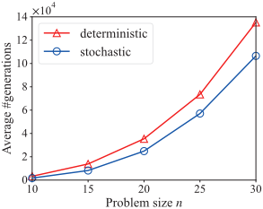
Specifically, we compare the number of generations of SMS-EMOA for solving OneJumpZeroJump, when the two population update methods are used, respectively. We set k to 2, the problem size n from 10 to 30, with a step of 5, and the population size µ=2(n-2k + 4), as suggested in Theorem 3. For each n, we run SMS-EMOA 1000 times independently, and record the number of generations until the Pareto front is found. Figure 3 shows the average number of generations of the 1000 runs. Note that the standard deviation is not included because it is very close to the mean and may make the figure look cluttered. We can observe that the stochastic population update method can bring a clear acceleration. Note that using non-dominated sorting and hypervolume indicator to rank solutions may also be time-consuming, thus the stochastic population update method which only requires to compare ⌊|P ∪ {x′ }|/2⌋ = ⌊(µ + 1)/2⌋ solutions in each generation can make the optimization procedure even faster.

6 Conclusion

In this paper, we challenge a common practice for a key component inMOEAs, population update, through rigorous theoretical analysis. Existing MOEAs always update the population in a deterministic manner, while we prove that for the well-known SMS-EMOA solving the bi-objective problem OneJumpZeroJump, introducing randomness into the population update procedure can significantly decrease the expected running time. Though being proved in a special case, this finding may hold more generally. In fact, our results echo some recent empirical studies [Liang et al., 2023], where a simple non-elitist MOEA (which is of the stochastic population update nature) has been found to outperform SMSEMOA on popular practical problems like the knapsack problem [Zitzler and Thiele, 1999] and NK-landscape [Aguirre and Tanaka, 2004].