
Self-Supervised Monocular Depth Estimation in the Dark: Towards Data Distribution Compensation
Proceedings of the Thirty-Third International Joint Conference on Artificial Intelligence. Main Track. Pages 1561-1569.
https://doi.org/10.24963/ijcai.2024/173
Keywords
- Computer Vision: CV: 3D computer vision
- Computer Vision: CV: Scene analysis and understanding
- Computer Vision: CV: Other
- Computer Vision: CV: Transfer, low-shot, semi- and un- supervised learning
Abstract
Nighttime self-supervised monocular depth estimation has received increasing attention in recent years. However, using night images for self-supervision is unreliable because the photometric consistency assumption is usually violated in the videos taken under complex lighting conditions. Even with domain adaptation or photometric loss repair, performance is still limited by the poor supervision of night images on trainable networks. In this paper, we propose a self-supervised nighttime monocular depth estimation method that does not use any night images during training. Our framework utilizes day images as a stable source for self-supervision and applies physical priors (e.g., wave optics, reflection model and read-shot noise model) to compensate for some key day-night differences. With day-to-night data distribution compensation, our framework can be trained in an efficient one-stage self-supervised manner. Though no nighttime images are considered during training, qualitative and quantitative results demonstrate that our method achieves SoTA depth estimating results on the challenging nuScenes-Night and RobotCar-Night compared with existing methods.
- [Azuma et al., 2001] Ronald Azuma, Yohan Baillot, Rein- hold Behringer, Steven Feiner, Simon Julier, and Blair MacIntyre. Recent advances in augmented reality. IEEE Computer Graphics and Applications, 21(6):34-47, 2001.
- [Bae et al., 2023] Jinwoo Bae, Sungho Moon, and Sunghoon Im. Deep digging into the generalization of self- supervised monocular depth estimation. In AAAI, 2023.
- [Brooks et al., 2019] Tim Brooks, Ben Mildenhall, Tianfan Xue, Jiawen Chen, Dillon Sharlet, and Jonathan T Barron. Unprocessing images for learned raw denoising. In CVPR, pages 11036-11045, 2019.
- [Caesar et al., 2020] Holger Caesar, Varun Bankiti, Alex H Lang, Sourabh Vora, Venice Erin Liong, Qiang Xu, Anush Krishnan, Yu Pan, Giancarlo Baldan, and Oscar Beijbom. nuscenes: A multimodal dataset for autonomous driving. In CVPR, pages 11621-11631, 2020.
- [Chen et al., 2018] Chen Chen, Qifeng Chen, Jia Xu, and Vladlen Koltun. Learning to see in the dark. In CVPR, pages 3291-3300, 2018.
- [Chen et al., 2019] Po-Yi Chen, Alexander H Liu, Yen- Cheng Liu, and Yu-Chiang Frank Wang. Towards scene understanding: Unsupervised monocular depth estima- tion with semantic-aware representation. In CVPR, pages 2624-2632, 2019.
- [Dai et al., 2022] Yuekun Dai, Chongyi Li, Shangchen Zhou, Ruicheng Feng, and Chen Change Loy. Flare7k: A phenomenological nighttime flare removal dataset. In NeurIPS, 2022.
- [Dosovitskiy et al., 2020] Alexey Dosovitskiy, Lucas Beyer, Alexander Kolesnikov, Dirk Weissenborn, Xiaohua Zhai, Thomas Unterthiner, Mostafa Dehghani, Matthias Min- derer, Georg Heigold, Sylvain Gelly, et al. An image is worth 16x16 words: Transformers for image recognition at scale. arXiv, 2020.
- [Eigen et al., 2014] David Eigen, Christian Puhrsch, and Rob Fergus. Depth map prediction from a single image using a multi-scale deep network. Advances in Neural In- formation Processing Systems, 27, 2014.
- [Feng et al., 2022] Hansen Feng, Lizhi Wang, Yuzhi Wang, and Hua Huang. Learnability enhancement for low-light raw denoising: Where paired real data meets noise model- ing. In ACM MM, pages 1436-1444, 2022. Godard et al., 2019]
- Clément Godard, Oisin Mac Aodha, Michael Firman, and Gabriel J Brostow. Digging into self- supervised monocular depth estimation. In ICCV, pages 3828-3838, 2019.
- [Goodman, 2005] Joseph W Goodman. Introduction to Fourier optics. Roberts and Company publishers, 2005.
- [Guizilini et al., 2020a] Vitor Guizilini, Rares Ambrus, Sudeep Pillai, Allan Raventos, and Adrien Gaidon. 3d packing for self-supervised monocular depth estimation. In CVPR, pages 2485-2494, 2020.
- [Guizilini et al., 2020b] Vitor Guizilini, Rui Hou, Jie Li, Rares Ambrus, and Adrien Gaidon. Semantically- guided representation learning for self-supervised monoc- ular depth. arXiv, 2020.
- [He et al., 2016] Kaiming He, Xiangyu Zhang, Shaoqing Ren, and Jian Sun. Deep residual learning for image recog- nition. In CVPR, pages 770-778, 2016.
- [Huang et al., 2021] Tao Huang, Songjiang Li, Xu Jia, Huchuan Lu, and Jianzhuang Liu. Neighbor2neighbor: Self-supervised denoising from single noisy images. In CVPR, pages 14781-14790, 2021.
- [Huang et al., 2022] Tao Huang, Songjiang Li, Xu Jia, Huchuan Lu, and Jianzhuang Liu. Neighbor2neighbor: A self-supervised framework for deep image denoising. IEEE Transactions on Image Processing, 31:4023-4038, 2022.
- [Joiner and Rosenblatt, 1971] Brian L Joiner and Joan R Rosenblatt. Some properties of the range in samples from tukey's symmetric lambda distributions. Journal of the American Statistical Association, 66(334):394-399, 1971.
- [Jung et al., 2021] Hyunyoung Jung, Eunhyeok Park, and Sungjoo Yoo. Fine-grained semantics-aware representa- tion enhancement for self-supervised monocular depth es- timation. In ICCV, pages 12642-12652, 2021.
- [Kakimoto et al., 2004] Masanori Kakimoto, Kaoru Mat- suoka, Tomoyuki Nishita, Takeshi Naemura, and Hiroshi Harashima. Glare generation based on wave optics. In PG, pages 133-140. IEEE, 2004.
- [Klingner et al., 2020] Marvin Klingner, Jan-Aike Termöhlen, Jonas Mikolajczyk, and Tim Fingscheidt. Self-supervised monocular depth estimation: Solving the dynamic object problem by semantic guidance. In ECCV, pages 582-600, 2020.
- [Lee et al., 2021] Seokju Lee, Sunghoon Im, Stephen Lin, and In So Kweon. Learning monocular depth in dynamic scenes via instance-aware projection consistency. In AAAI, pages 1863-1872, 2021.
- [Li et al., 2021] Hanhan Li, Ariel Gordon, Hang Zhao, Vin- cent Casser, and Anelia Angelova. Unsupervised monoc- ular depth learning in dynamic scenes. In CoRL, pages 1908-1917, 2021.
- [Lipson et al., 2010] Ariel Lipson, Stephen G Lipson, and Henry Lipson. Optical physics. Cambridge University Press, 2010.
- [Liu et al., 2021] Lina Liu, Xibin Song, Mengmeng Wang, Yong Liu, and Liangjun Zhang. Self-supervised monocu- lar depth estimation for all day images using domain sep- aration. In ICCV, pages 12737-12746, 2021.
- [Luidolt et al., 2020] Laura R Luidolt, Michael Wimmer, and Katharina Krösl. Gaze-dependent simulation of light perception in virtual reality. IEEE Transactions on Visual- ization and Computer Graphics, 26(12):3557-3567, 2020.
- [Lyu et al., 2021] Xiaoyang Lyu, Liang Liu, Mengmeng Wang, Xin Kong, Lina Liu, Yong Liu, Xinxin Chen, and Yi Yuan. Hr-depth: High resolution self-supervised monocular depth estimation. In AAAI, pages 2294-2301, 2021.
- [Ma et al., 2022] Jingyuan Ma, Xiangyu Lei, Nan Liu, Xian Zhao, and Shiliang Pu. Towards comprehensive represen- tation enhancement in semantics-guided self-supervised monocular depth estimation. In ECCV, pages 304-321, 2022.
- [Maddern et al., 2017] Will Maddern, Geoffrey Pascoe, Chris Linegar, and Paul Newman. 1 year, 1000 km: The oxford robotcar dataset. The International Journal of Robotics Research, 36(1):3-15, 2017.
- [Menze and Geiger, 2015] Moritz Menze and Andreas Geiger. Object scene flow for autonomous vehicles. In CVPR, pages 3061-3070, 2015.
- [Nadon et al., 2018] Félix Nadon, Angel J Valencia, and Pierre Payeur. Multi-modal sensing and robotic manip- ulation of non-rigid objects: A survey. Robotics, 7(4):74, 2018.
- [Petrovai and Nedevschi, 2022] Andra Petrovai and Sergiu Nedevschi. Exploiting pseudo labels in a self-supervised learning framework for improved monocular depth estima- tion. In CVPR, pages 1578-1588, 2022.
- [Phong, 1975] Bui Tuong Phong. Illumination for com- puter generated pictures. Communications of the ACM, 18(6):311-317, 1975.
- [Ruyten, 1999] Wim Ruyten. Smear correction for frame transfer charge-coupled-device cameras. Optics Letters, 24(13):878-880, 1999.
- [Spencer et al., 2023] Jaime Spencer, C Stella Qian, Chris Russell, Simon Hadfield, Erich Graf, Wendy Adams, An- drew J Schofield, James H Elder, Richard Bowden, Heng Cong, et al. The monocular depth estimation challenge. In WACV, pages 623-632, 2023.
- [Tang et al., 2013] Shuai Tang, Xiaoyu Wang, Xutao Lv, Tony X Han, James Keller, Zhihai He, Marjorie Skubic, and Shihong Lao. Histogram of oriented normal vectors for object recognition with a depth sensor. In ACCV, pages 525-538. Springer, 2013.
- [Vankadari et al., 2020] Madhu Vankadari, Sourav Garg, Anima Majumder, Swagat Kumar, and Ardhendu Behera. Unsupervised monocular depth estimation for night-time images using adversarial domain feature adaptation. In ECCV, pages 443-459, 2020.
- [Vankadari et al., 2023] Madhu Vankadari, Stuart Golodetz, Sourav Garg, Sangyun Shin, Andrew Markham, and Niki Trigoni. When the sun goes down: Repairing photomet- ric losses for all-day depth estimation. In Conference on Robot Learning, pages 1992-2003, 2023.
- [Wagstaff and Kelly, 2021] Brandon Wagstaff and Jonathan Kelly. Self-supervised scale recovery for monocular depth and egomotion estimation. In IROS, pages 2620-2627, 2021.
- [Wang et al., 2021] Kun Wang, Zhenyu Zhang, Zhiqiang Yan, Xiang Li, Baobei Xu, Jun Li, and Jian Yang. Reg- ularizing nighttime weirdness: Efficient self-supervised monocular depth estimation in the dark. In ICCV, pages 16055-16064, 2021.
- [Wei et al., 2020] Kaixuan Wei, Ying Fu, Jiaolong Yang, and Hua Huang. A physics-based noise formation model for extreme low-light raw denoising. In CVPR, pages 2758- 2767, 2020.
- [Wei et al., 2021] Kaixuan Wei, Ying Fu, Yinqiang Zheng, and Jiaolong Yang. Physics-based noise modeling for ex- treme low-light photography. IEEE Transactions on Pat- tern Analysis and Machine Intelligence, 2021.
- [Xue et al., 2020] Feng Xue, Guirong Zhuo, Ziyuan Huang, Wufei Fu, Zhuoyue Wu, and Marcelo H Ang. Toward hier- archical self-supervised monocular absolute depth estima- tion for autonomous driving applications. In IROS, pages 2330-2337, 2020.
- [Yan et al., 2021] Jiaxing Yan, Hong Zhao, Penghui Bu, and YuSheng Jin. Channel-wise attention-based network for self-supervised monocular depth estimation. In 3DV, pages 464-473, 2021.
- [Zhang et al., 2021] Yi Zhang, Hongwei Qin, Xiaogang Wang, and Hongsheng Li. Rethinking noise synthesis and modeling in raw denoising. In ICCV, pages 4593-4601, 2021.
- [Zhao et al., 2020] Chaoqiang Zhao, Qiyu Sun, Chongzhen Zhang, Yang Tang, and Feng Qian. Monocular depth es- timation based on deep learning: An overview. Science China Technological Sciences, 63(9):1612-1627, 2020.
- [Zhao et al., 2022a] Chaoqiang Zhao, Yang Tang, and Qiyu Sun. Unsupervised monocular depth estimation in highly complex environments. IEEE Transactions on Emerging Topics in Computational Intelligence, 6(5):1237-1246, 2022.
- [Zhao et al., 2022b] Chaoqiang Zhao, Youmin Zhang, Mat- teo Poggi, Fabio Tosi, Xianda Guo, Zheng Zhu, Guan Huang, Yang Tang, and Stefano Mattoccia. Monovit: Self- supervised monocular depth estimation with a vision trans- former. In 3DV, 2022.
- [Zhou et al., 2017] Tinghui Zhou, Matthew Brown, Noah Snavely, and David G Lowe. Unsupervised learning of depth and ego-motion from video. In CVPR, pages 1851- 1858, 2017.
References were extracted automatically from the PDF and may contain errors.
Full text extracted automatically from the PDF; figures, tables and equations may differ. The PDF is the version of record.
1 Introduction
Monocular depth estimation plays a key role in several applications, such as augmented reality [Azuma et al., 2001], autonomous driving [Menze and Geiger, 2015] and robotic manipulation [Nadon et al., 2018]. With the usage and development of neural networks, like Convolutional Neural Network [He et al., 2016] and Vision Transformer [Dosovitskiy et al., 2020], deep-learning approaches present impressive results in this task [Zhao et al., 2020]. Since the self-supervised framework does not require numerous costly depth-image pairs during training, it has achieved increasing attention in recent years. Instead of using ground truth depth labels, the spatial and temporal geometric constraints from images are constructed in the self-supervised framework to supervise the training process. The photometric consistency assumption is used to build up the main constraint (i.e., the photometric loss) of self-supervision. Results in [Godard et al., 2019;
MonoFormer G: Ours Ours
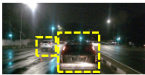
Figure 1: Nighttime monocular estimation results of different self-supervised frameworks. Compared with existing domain adaptation-based methods RNW [Wang et al., 2021] and ADDS [Liu et al., 2021] and recent large model MonoFormer [Bae et al., 2023], our result shows superior performance.
Zhao et al., 2022b; Guizilini et al., 2020a; Lyu et al., 2021] show the effectiveness of classic self-supervised training on day scenes.
While for nighttime scenes, the complex lighting conditions lead to significant photometric inconsistency within night-image sequences. And it causes divergence of training. To alleviate this problem, domain adaptation-based methods and photometric loss repair-based methods are proposed recently. The domain adaptation-based methods [Liu et al., 2021; Wang et al., 2021; Zhao et al., 2022a; Vankadari et al., 2020] apply extra adversarial loss or domain transfer network to make the depth model learn to decouple structure information and interfering elements. Meanwhile, the photometric loss repair-based method [Vankadari et al., 2023] utilizes additional trainable and trained parts to complement the daytime photometric loss. Although these methods show improved results compared to the classical self-supervised framework [Godard et al., 2019], their performance is still limited by the poor transfer quality of the image transfer model or the incomplete elimination of lighting effects in the photometric loss.
In this paper, we suspend the direct application of nighttime images during training since they are an inappropriate source of self-supervision. Our goal is to train a night depth network that does not see night images during training, but only day images, in a self-supervised manner. We achieve such a design by extracting some principal day-night dissimilarities and using physical priors to compensate for the day-image distribution. Focusing on the difference in lighting conditions, the dissimilarities in photometric and noise
RNW
ADDS
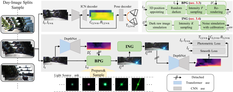
distribution are located as two key components. Then, we build up corresponding modules for simulation. Considering the wave optics/diffraction effect of light sources as well as reflections, we propose Brightness Peak Generator (BPG) to model the difference in photometric distribution. Based on the shot-read noise model, we build up Imaging Noise Generator (ING) to model nighttime noise distribution. The joint application of BPG and ING together with the day-image distribution results in a fused distribution that has a photometric and noise distribution close to the night images. The fused distribution is randomly sampled and used for the training of the depth network. As shown in Fig. 1, though no night image is seen during training, our method still achieves superior performance compared to existing nighttime methods.
Our main contributions are summarized as follows: (I) We propose a nighttime monocular depth training framework that use day image pairs as the stable source of self-supervision. (II) Our training framework requires no night images during training. We accomplish this design by day-to-night data distribution compensation. (III) Photometric and noise distributions are located as two key day-night differences. Using physical priors, we propose two simple but effective modules to model the differences in these distributions accordingly. Our presented method achieves SoTA performance on the challenging nuScenes-Night and RobotCar-Night dataset, though no nighttime images are used in our training framework.
2 RelatedWork
Estimating depth from a single image is an ill-posed problem, and deep learning-based frameworks address this challenge in an end-to-end manner and show promising performance [Zhao et al., 2020]. Considering the availability of precise depth labels in the real world, self-supervised solutions [Zhou et al., 2017; Godard et al., 2019] propose to use geometric constraints between image sequences instead of depth labels during training and received increasing attention recently [Zhao et al., 2020].
Daytime Self-Supervised Framework
Considering the geometric constraints between temporal images, SfMLearner [Zhou et al., 2017] is proposed to use monocular image sequences to train the monocular depth network. During training, a depth network and a pose network are designed to construct the geometric relationship between images, and a view reconstruction loss is used to supervise the training process. Based on this framework, many works are proposed to handle the challenges caused by occlusions [Godard et al., 2019], dynamic objects [Li et al., 2021; Lee et al., 2021] and scale ambiguity [Xue et al., 2020; Wagstaff and Kelly, 2021; Petrovai and Nedevschi, 2022]. Meanwhile, some methods [Chen et al., 2019; Guizilini et al., 2020b; Jung et al., 2021; Ma et al., 2022; Klingner et al., 2020] introduce and fuse semantic information into training to improve the depth estimation performance. Many methods [Zhao et al., 2022b; Lyu et al., 2021; Guizilini et al., 2020a; Yan et al., 2021] try to improve the depth estimation from the aspect of network architectures. Most recently, MonoViT [Zhao et al., 2022b; Spencer et al.,
2023] and MonoFormer [Bae et al., 2023] combine both CNN and Transformer blocks to learn both local and global features of images, and their results on unseen scenes show the convincing generalization ability of their network.
Nighttime Self-Supervised Framework
Although the above methods show satisfactory depth estimation results, for nighttime scenes, such methods usually failed during training and testing because of significant day-night distribution differences. To estimate in the night, many methods [Liu et al., 2021; Wang et al., 2021; Zhao et al., 2022a; Vankadari et al., 2020] are proposed to address the challenge through domain adaptation or photometric loss restoration. ADFA [Vankadari et al., 2020] succeeds in nighttime training by domain adaptation on feature space. They train a nighttime DepthNet encoder to learn daytime-like features with adversarial loss. ITDFA [Zhao et al., 2022a] and ADDS [Liu et al., 2021] utilize the image transfer-based domain adaptation framework. Based on the transferred image pairs, ITDFA [Zhao et al., 2022a] constrains the training process on both feature and output spaces, while ADDS [Liu et al., 2021] tries to learn a better decoupling of the private and invariant domains. However, the performance of ITDFA and ADDS is restricted by the image transfer quality. Defects in the texture can cause the prediction missing structural details. In RNW [Wang et al., 2021], an improved priors-based domain adaptive on output space is used to regularize nighttime photometric outliers. However, the significant illumination inconsistency within poor-quality image sequences is still out of regularization and causes performance degradation. WSGD [Vankadari et al., 2023] is the first one-stage method that directly trains their proposed framework on nighttime image splits. It introduces an Illuminating Change Net, a Residual Flow Net and a frozen Denoise Net [Huang et al., 2021; Huang et al., 2022] into monocular training. Instead of applying domain adaptation, they utilize extra trainable and trained parts to refine the photometric loss.
Though these methods show nighttime monocular depth estimation ability, low light and complex light in nighttime scenes still affect the photometric-based self-supervised training process. Meanwhile, the benefits of the image transfer model are limited. In contrast, our method performs data distribution compensation on day images and does not suffer from the poor self-supervision of night images.
3 Approach
3.1 Data Distribution Compensation Framework Compensation and Sample
To enable the depth network that sees no night image but generalizes well to different night scenes, and to take advantage of the stable self-supervision of day images, we make a compensation on the day-image distribution with day-night differences:
where Pd and Pn represent the day-image and night-image distributions, Pshift donates the distribution difference between them, ˜ Pshift refers to the simulation of some key differences, and I LRN t indicates one sample from the fused distribution.
Physical Priors or Image Transfer
Either physical priors or image transfer technology can be used to build the fused distribution, Pd + ˜ Pshift. Though vivid fake night images could be transferred with solid backbones and properly partitioned training sets, some key differences (e.g., differences in photometric and noise distribution) between day and night could be underestimated in the image transfer network because no corresponding constraint is made during their training.
Different from image transfer technology, the use of physical priors is more controllable, directional and explainable. It's also efficient because it doesn't require additional training stages or excessive memory costs. Thus, we use physical priors to model ˜ Pshift. In addition, focusing on lighting conditions, we analyze key day-night differences in Section 3.2 and describe their modeling in Section 3.3 and Section 3.4.
Self-Supervised Training
The proposed framework is trained in a self-supervised manner. Following [Godard et al., 2019; Zhao et al., 2022b], the combination of photometric loss and edge-aware smooth loss is used as the main supervision during training, and the framework is shown in Fig. 2. We use the same TransformerCNN hybrid network in MonoViT [Zhao et al., 2022b] as our DepthNet because of its good performance. Besides, inspired by [Vankadari et al., 2023], we further consider the potential illuminating changes between images, and the Illuminating Change Net (ICN) is introduced to predict the linear per-pixel illuminating change Ct,t+n and Bt,t+n. In addition, to avoid poor self-supervision, we make a simple decoupling at the input stage, and the sampled I LRN t is only applied to the input of the depth network.
3.2 Day-Night Image Differences Analysis
Objects (cars, trees, pedestrians, streets, sky, etc.) in day and night scenes share the same internal properties and similar distributions, but when captured objects on images by camera sensors, the reactions of objects and sensors in different lighting conditions result in dissimilarities in photometric and noise distribution.
Photometric Distribution
For daytime scenes, the parallel white light from the sun illuminates the scene and reflects the color of objects. The color, intensity and direction of the light are almost exactly the same between images, and the evenly distributed brightness matches the texture gradient of the objects well so that the photometric consistency assumption can be built on daytime images [Godard et al., 2019; Zhao et al., 2022a; Vankadari et al., 2023]. While for nighttime scenes, dynamic/static light sources together with different light colors result in a highly complex and nonuniform photometric distribution on the scenes. Besides, on the image coordinates, the correspondence between the brightness gradient and the textures fails because the significant brightness peaks caused by the light sources overwhelm the texture gradient of scenes.
Imaging Noise
Since cameras are not perfect imaging device, it has a limited dynamic range and introduces noise at most stages of the imaging process [Chen et al., 2018]. At night, the camera adjusts the system gain to compensate for the lower number of input photons, so noise is amplified and appears more pronounced in the raw image [Wei et al., 2020; Wei et al., 2021; Zhang et al., 2021]. When the noise intensity exceeds the denoising capability of the Image Sensor Processor (ISP) [Chen et al., 2018; Brooks et al., 2019], it will not be negligible in the output image. Heavy noise distorts the local distribution and creates fake textures on both foreground and background, and such fake textures confuse the daytime depth model during testing.
3.3 Photometric DistributionModeling
In this part, we model the nonuniform photometric distribution at night by adding additional light sources. The wave optics/diffraction effect of light source imaging and reflections are considered in the sampling. Since it makes peaks of brightness in the original image plane, we call it Brightness Peak Generator (BPG).
Light Source Sample
Due to the diffraction/wave optics effects [Lipson et al., 2010; Goodman, 2005], when a point light is viewed through an aperture that is not an ideal circle or a lens that is stained or scratched, the imaging results of the light source will be a combination of glare, streak, and shimmer, instead of a dot [Dai et al., 2022; Kakimoto et al., 2004]. In computer graphics, some methods [Kakimoto et al., 2004; Luidolt et al., 2020] approximate this optical phenomenon by using the 2D Fourier transform, but the output is uncontrollable and the cost is expensive. Therefore, instead of simulating the light source image directly, we construct a light source bank based on Flare7K [Dai et al., 2022] dataset, which is the only light source dataset with 7000 samples.
When applied, BPG randomly samples a single image from the light source bank. Then, the image will be scaled to the standard size which is determined by the long side of It (A square whose sides are equal to the long side of It ). Simple image augmentation is further applied to expand the number of light source images. The scaled and augmented light source image is used as the standard light source image LS.
3D Position of Light Source
The sampled light source is assumed to be randomly distributed in the scene. We do not model the location because it is costly to include precise segmentation information in our training which requires large trained models.
Firstly, a 2D coordinate pi is randomly appointed as the location of the light source. We limit the depth of it, zi, with the predicted scale depth map (discussed latter in this section). A up range with higher priority was manually set to 25m as farther light sources produce almost invisible reflection images. Then, the appointed 3D position will be:
Random Darken
The above light source imaging LS cannot produce significant peaks of brightness on the image because the daytime image is usually well-lit with high brightness. To efficiently improve the role of LS on the photometric distribution, a simple random darkening operation is applied. The illumination scale rate is set to follow uniform distribution, i.e. sd ∼ U(0.4, 1).
BPG Intensity F
We use the product of the light sources number NF and a resize scale rate sF as the BPG Intensity F . To enrich outputs while avoiding numerous aggressive results, a log uniform distribution is applied to select NF and F:
Following Flare7K [Dai et al., 2022], BPG adds the light source within the gamma range of gf ∼ U(1.8, 2.2). The sampled image on current stage, I L t , will be
Re-Rendering
Reflections are also one of the important representations of light sources in the scene, affecting the color and texture of objects in the image plane. Thus, we build up a re-rendering submodule within BPG for compensation.
With limited and biased information (3D structure, surface normal, material, etc) about the scene, we find the popular used Phong illumination model [Phong, 1975] effective. Note that only the predicted unscaled depth map D′t , the color image It, and the camera intrinsic KI are used in the rerendering submodule.
Since the predicted depth map D′t differs from the realworld values by a scale factor s, following [Xue et al., 2020; Petrovai and Nedevschi, 2022], we use the unscaled camera height to predict the scale factor. By predicting surface normal fromD′t , the unscaled camera height H′c is estimated thereafter. Thus, the scale factor will be
where Hc is the actual camera height. With the predicted scale factor s, the structured point cloud P can be calculated with
We then use predicted depth map D′t to calculate our surface normal [Tang et al., 2013] and directly use the color image It to extract coarse material information. Using the structured point cloud P, surface normal, coarse material of objects, the color of light source together with the appointed position, Pi (Eq. 2), we can calculate the reflection image I R i with simple but effective Phong illumination model [Phong, 1975]. The sampled image on current stage, I LR t , will be:
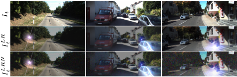
The detailed calculation of I R i is shown in the supplementary, and we give some examples of re-rendering in Fig. 3.
3.4 Imaging Noise Modeling
Heavy noise at night corrupts the local distribution and makes fake textures. Based on the shot-read noise model [Wei et al., 2020; Wei et al., 2021], we build our Imaging Noise Generator (ING) using color images as input.
Noise Model
For a camera imaging system, if without Image Signal Processor (ISP), a linear model can generally formulate the digit sensor raw image [Wei et al., 2020; Feng et al., 2022]:
where C is the number of photon, K donates the overall system gain, and N refers to the summation of all physical noise. In the physical model base image denoising [Wei et al., 2020; Wei et al., 2021; Zhang et al., 2021], the overall noise N, is roughly separated into shot noise Np and read noise Nread:
Here, Shot noise is caused by the collection uncertainty of photons, which follows
with P indicating Poisson distribution.
Meanwhile, the composition of read noise is more complex, and Nread is usually assumed to follow a bellshape distribution e.g. Gaussian distribution, N(0, σN) and Tukey lambda distribution [Joiner and Rosenblatt, 1971], TL(λTL; 0, σTL). TL is a distribution family that can fit many bell-shaped distributions, and λTL is used to control the shape. Applying the linear least squares method, the system gains K and the variance of the distribution are considered to be linear in the logarithmic domain [Wei et al., 2020]:
with aN(aTL) and bN(bTL) being the approximating linear parameters and ˆσN(ˆσTL) donating the standard deviation of the unbiased estimation. In ELD [Wei et al., 2020], different kinds of digit sensors are calibrated with Gaussian distribution and Tukey lambda distribution respectively and ING randomly samples the calibrations to generate read noise Nread.
From RGB to Simulated Dark Raw Image RLR t
In ELD, shot noise Np is applied on the number of photons R/K while read noise Nread on raw image R. However, raw images or the exact inverse ISP are not available in most daytime datasets. The simplest ISP includes white balance, binning, denoising, color collection and gamma compression [Chen et al., 2018; Brooks et al., 2019]. Fortunately, except for denoising and gamma compression, rest operations can be viewed as approximately linear processes. We consider the gamma compression in ING as it's strongly nonlinear. Following ELD, we set gn = 1/2.2.
To simulate the low photon count C in the dark, a light scale factor sn is proposed follows U(100, 300) [Wei et al., 2020]. Then, the simulated raw image will be
where sbit denotes quantization factor equals to 2bit - 1.
ING Intensity K
According to Eq. 9, Eq. 11 and Eq. 12, system gain K has a positive relationship with the noise intensity. Therefore, we appoint K as ING Intensity. Similar in BPG, we make ING Intensity following the log uniform:
Finally, with the simulated raw image RLR t , the sampled shot noise Np and read noise Nread, the output of ING will be
Fig. 4 visualizes some examples of I LRN t .
4 Experiments
4.1 Dataset
We construct the self-supervised training process on the widely used KITTI dataset, and following [Godard et al., 2019; Zhao et al., 2022b], the KITTI Eigen training split [Eigen et al., 2014] is used as the training set due to its high-quality images, and we also regard it as our basic day-image distribution.
For evaluation, we use the nuScenes-Night test split from RNW [Wang et al., 2021] and the RobotCar-Night test split proposed in ADDS [Liu et al., 2021]. And we also follow the same pre-cropping method proposed in their work.
4.2 Effective Test
Comparisons
We mainly compare our results with four SoTA methods i.e. DA (Domain adaptation): RNW [Wang et al., 2021], DA: ADDS [Liu et al., 2021], DA: ITDFA [Zhao et al., 2022a] and DT (Direct training): WSGD [Vankadari et al., 2023] on nuScenes-Night and RobotCar-Night, respectively. To make a fair comparison, all methods apply the same TransformerCNN hybrid backbone [Zhao et al., 2022b] if no further explanation is made. We also provide the G (Generalize to test set) version result of each DA method for further comparisons. In addition, we will release the code upon acceptance.
| Type | Method | Train on | Train Res. | Max depth | ABS rel↓ | Sq rel↓ | RMSE↓ | RMSE log↓ | δ1 ↑ | δ2 ↑ | δ3 ↑ |
|---|---|---|---|---|---|---|---|---|---|---|---|
| Test on nuScenes-Night | |||||||||||
| DT | MonoViT[Zhao et al., 2022b] WSGD[Vankadari et al., 2023] | N d&n | 640 × 320 | 60 | 1.726 | 93.031 | 30.321 | 2.183 | 0.143 | 0.291 | 0.437 |
| N d&n | 640 × 320 | 60 | 0.663 | 9.573 | 15.200 | 0.755 | 0.199 | 0.388 | 0.567 | ||
| DA | ITDFA[Zhao et al., 2022a] RNW[Wang et al., 2021]† RNW[Wang et al., 2021] | N d&n | 640 × 320 | 60 | 0.337 | 4.511 | 10.118 | 0.403 | 0.515 | 0.767 | 0.890 |
| N d&n | 768 × 384 | 60 | 0.315 | 3.792 | 9.641 | 0.403 | 0.508 | 0.778 | 0.896 | ||
| N d&n | 640 × 320 | 60 | 0.341 | 5.516 | 11.152 | 0.406 | 0.531 | 0.789 | 0.902 | ||
| N d&n | 640 × 320 | 60 | 0.299 | 4.790 | 10.372 | 0.371 | 0.620 | 0.814 | 0.907 | ||
| G | ADDS[Liu et al., 2021] WSGD[Vankadari et al., 2023] ITDFA[Zhao et al., 2022a] RNW[Wang et al., 2021] ADDS[Liu et al., 2021] MonoFormer[Bae et al., 2023]‡ MonoViT[Zhao et al., 2022b] | R d&n | 640 × 320 | 60 | 0.314 | 3.567 | 10.058 | 0.408 | 0.520 | 0.758 | 0.881 |
| R d&n | 640 × 320 | 60 | 0.362 | 3.760 | 10.252 | 0.441 | 0.418 | 0.702 | 0.867 | ||
| R d&n | 640 × 320 | 60 | 0.376 | 4.732 | 11.193 | 0.506 | 0.451 | 0.712 | 0.835 | ||
| R d&n | 640 × 320 | 60 | 0.322 | 4.401 | 10.584 | 0.397 | 0.527 | 0.786 | 0.892 | ||
| K | 768 × 256 | 60 | 0.307 | 3.591 | 10.162 | 0.413 | 0.521 | 0.762 | 0.872 | ||
| K | 768 × 256 | 60 | 0.348 | 4.144 | 11.086 | 0.473 | 0.417 | 0.708 | 0.843 | ||
| Ours | K | 768 × 256 | 60 | 0.259 | 3.147 | 8.547 | 0.344 | 0.641 | 0.850 | 0.928 | |
| Test on RobotCar-Night | |||||||||||
| DT | MonoViT[Zhao et al., 2022b] | R d&n | 640 × 320 | 40 | 0.513 | 13.558 | 9.867 | 0.479 | 0.588 | 0.846 | 0.918 |
| WSGD[Vankadari et al., | 2023] R d&n | 640 × 320 | 40 | 0.202 | 1.835 | 5.985 | 0.231 | 0.737 | 0.934 | 0.977 | |
| DA | ITDFA[Zhao et al., 2022a] ADDS[Liu et al., 2021]† ADDS[Liu et al., 2021] | R d&n | 640 × 320 | 40 | 0.266 | 3.010 | 8.293 | 0.287 | 0.567 | 0.888 | 0.962 |
| R d&n | 512 × 256 | 40 | 0.233 | 2.344 | 6.859 | 0.270 | 0.631 | 0.908 | 0.962 | ||
| R d&n | 640 × 320 | 40 | 0.209 | 2.179 | 6.808 | 0.254 | 0.704 | 0.918 | 0.965 | ||
| RNW[Wang et al., 2021] | R d&n | 640 × 320 | 40 | 0.197 | 1.789 | 5.896 | 0.234 | 0.742 | 0.930 | 0.972 | |
| G | ITDFA[Zhao et al., 2022a] ADDS[Liu et al., 2021] RNW[Wang et al., 2021] MonoFormer[Bae et al., 2023]‡ MonoViT[Zhao et al., 2022b] | N d&n | 640 × 320 | 40 | 0.302 | 3.692 | 8.642 | 0.327 | 0.548 | 0.852 | 0.938 |
| N d&n | 640 × 320 | 40 | 0.265 | 3.651 | 8.700 | 0.309 | 0.640 | 0.870 | 0.945 | ||
| N d&n | 640 × 320 | 40 | 0.237 | 2.958 | 8.187 | 0.298 | 0.683 | 0.885 | 0.948 | ||
| K | 768 × 256 | 40 | 0.289 | 2.893 | 7.468 | 0.302 | 0.543 | 0.873 | 0.964 | ||
| K | 768 × 256 | 40 | 0.253 | 2.044 | 6.208 | 0.269 | 0.572 | 0.908 | 0.977 | ||
| Ours | K | 768 × 256 | 40 | 0.210 | 1.515 | 5.386 | 0.238 | 0.676 | 0.936 | 0.980 | |
| Method | ABS rel ↓ | Sq rel ↓ | RMSE ↓ | RMSE log ↓ | δ1 ↑ | δ2 ↑ | δ3 ↑ |
|---|---|---|---|---|---|---|---|
| Test on nuScenes-Night | |||||||
| Baseline | 0.327 | 3.740 | 10.703 | 0.448 | 0.451 | 0.733 | 0.855 |
| BPG Only | 0.264 | 2.956 | 9.209 | 0.371 | 0.581 | 0.813 | 0.914 |
| ING Only | 0.268 | 3.177 | 9.397 | 0.371 | 0.588 | 0.807 | 0.909 |
| Full Method | 0.259 | 3.147 | 8.547 | 0.344 | 0.641 | 0.850 | 0.928 |
| Test on RobotCar-Night | |||||||
| Baseline | 0.242 | 1.882 | 5.962 | 0.261 | 0.600 | 0.915 | 0.979 |
| BPG Only | 0.216 | 1.827 | 5.986 | 0.248 | 0.686 | 0.920 | 0.976 |
| ING Only | 0.238 | 1.817 | 5.882 | 0.257 | 0.620 | 0.920 | 0.980 |
| Full Method | 0.210 | 1.515 | 5.386 | 0.238 | 0.676 | 0.936 | 0.980 |
Evaluation on nuScenes-Night
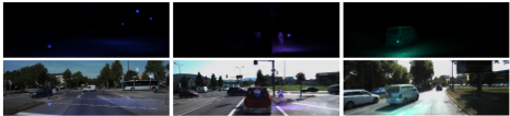
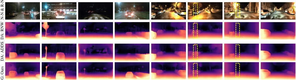
As shown in Fig. 5, due to the weak interference of ISP on the digit raw, wave optics/diffraction effects are evident, and the imaging noise is also visible. Though it provides more realistic imaging compared to that in RobotCar-Night, it introduces further disadvantages in the photometric loss. Thus, two DT methods strongly diverge on this dataset.
Meanwhile, our method generalizes well to these unseen nighttime scenes and outperforms all DA methods though no image from nuScenes dataset is used in our training. Besides, our method makes a 13.3% improvement on ABS rel and 17.6% improvement on RMSE compared to the second-best approach (DA:ADDS).
As shown in the upper portion of Fig. 5, our method outperforms the second-best and third-best method by a margin with much fewer prediction outliers. In addition, our method provides reasonable depth prediction for both dim scenes and bright scenes.
Evaluation on RobotCar-Night
As shown in Fig. 5, the strong corrective effect of ISP in RobotCar-Night results in a cleaner image plane compared to that in nuScnce-Night. The light sources do not image streak and there is little noise in the sky. Here, we use RobotCarNight to test the effectiveness of our method when the wave optics effect and noise are not significant.
The bottom half of Table 1 shows quantitative results on RobotCar-Night. Our result still outperforms the second-best method (DA: RNW) by 15.3% in Sq rel and 8.7% in RMSE, despite the reduction in ABS rel. Given that Sq rel and RMSE is sensitive to outlier points, the comparison suggests that the DepthNet trained by our framework prefers to make fewer prediction outliers rather than take the risk of making potentially more accurate but radical predictions.
In the bottom portion of Fig. 5, we mark the smearing regions [Ruyten, 1999] that are caused by the CCD (Chargecoupled-Device) imaging errors instead of the wave optics/diffraction effect. Our method gives a more accurate prediction in these regions compared to ADDS and RNW, which shows the robustness of our method.
In addition, the comparisons between the top and bottom halves of Fig. 5 and Table 1 suggest that the performance of DA: ADDS, DA: RNW and DT: WSGD degrades on nuScenes-Night. It also reveals that domain adaptation-based and photometric loss repair-based methods are still limited by the quality of night images. Meanwhile, using the same backbone of DepthNet, our method maintains convincing results on both nuScenes-Night and Robotcar-Night, although no image from these two datasets is used during training.
Comparison of G Results
In Table 1, we also provide the G results of domain adaptation-based methods. Their decrease in accuracy presents that these methods generalize poorly to unseen night scenes, while our approach does not suffer from such a drawback, and note that no specific nighttime dataset is used as the target dataset during our training.
In our supplementary material, we provide additional tests on nuScenes-Day and Robotcar-Day, give a complete qualitative comparison on nuScenes-Night/nuScenes-Day and RobotCar-Night/RobotCar-Day, and offer additional visual results on other nighttime datasets to further prove the effectiveness of our method.
4.3 Ablation Test on Pre-Processing Contribution of Each Part
Table 2 shows the contributions of each pre-processing part. The comparison of different self-supervised training approaches is left to the supplementary material to further prove the effectiveness of our training framework.
In nuScenes-Night, compared with the baseline, BPG improves ABS rel by 19.3% and RMSE by 14.0%, and ING improves ABS rel by 18.0% and RMSE by 9.1%. Besides, the joint application of BPG and ING achieves the best scores with 20.8% improvement on ABS rel, 20.1% on RMSE and 35.3% on δ1. For RobotCar-Night, the joint application of BPG and ING still achieves a significant boost with 13.2% on ABS rel and 9.7% on RMSE.
In addition, Table 2 shows that the joint application of BPG and ING significantly improves RMSE (7.2% in nuScenecNight and 8.4% in RobotCar-Night compared to the secondbest), suggesting that our data distribution compensation benefits on the prediction robustness.
Ablating Into BPG and ING
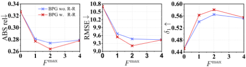
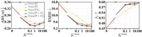
Fig. 6 visualizes a further ablation study on our BPG. The experiments show that our re-rendering submodule plays an important role within BPG. Besides, BPG achieves the best result when F max is set to 2. Meanwhile, Fig. 7 presents a detailed ablation on our ING. Apart from the standard groups (P + TL and P + N ), we also test P, N and TL (Eq. 10, Eq. 11 and Eq. 12) alone. Taken the three metrics shown in Fig. 7 together, P + TL and P + N still achieve better performance. According to Fig. 7(b) and Fig. 7(c), P + TL maintains the most consistent performance as Kmax changes. In addition, we set Kmax to 1 as ABS rel increases after Kmax is greater than 1, which suggests that inappropriately high intensity of ING will lead to overly conservative predictions.
5 Conclusion
This paper proposes a self-supervised monocular depth training framework for nighttime, which requires no nighttime image during training but day-to-night data distribution compensation. Focusing on day-night lighting differences, dissimilarities in photometric and noise distribution are located as two key components. We model the difference in corresponding distributions with the proposed BPG and ING. The samples from the fused distribution are used for the training of the depth network. Although no nighttime images were used during training, our model shows a more convincing performance than those nighttime frameworks, and our presented self-supervised method provides a new and feasible way for the nighttime monocular depth estimation task.
Acknowledgments
This work was supported in part by the National Key Research and Development Program of China under Grant 2021YFB1714300, in part by the National Natural Science Foundation of China under Grant 62233005, in part by the National Natural Science Foundation of China under Grant 62203173, in part by the Program of Introducing Talents of Discipline to Universities through the 111 Project under Grant B17017 and Shanghai AI Lab.
@inproceedings{ijcai2024p173,
  title     = {Self-Supervised Monocular Depth Estimation in the Dark: Towards Data Distribution Compensation},
  author    = {Yang, Haolin and Zhao, Chaoqiang and Sheng, Lu and Tang, Yang},
  booktitle = {Proceedings of the Thirty-Third International Joint Conference on
               Artificial Intelligence, {IJCAI-24}},
  publisher = {International Joint Conferences on Artificial Intelligence Organization},
  editor    = {Kate Larson},
  pages     = {1561--1569},
  year      = {2024},
  month     = {8},
  note      = {Main Track},
  doi       = {10.24963/ijcai.2024/173},
  url       = {https://doi.org/10.24963/ijcai.2024/173},
}
TY - CPAPER TI - Self-Supervised Monocular Depth Estimation in the Dark: Towards Data Distribution Compensation AU - Yang, Haolin AU - Zhao, Chaoqiang AU - Sheng, Lu AU - Tang, Yang T2 - Proceedings of the Thirty-Third International Joint Conference on Artificial Intelligence, IJCAI-24 PB - International Joint Conferences on Artificial Intelligence Organization PY - 2024 SP - 1561 EP - 1569 DO - 10.24963/ijcai.2024/173 UR - https://doi.org/10.24963/ijcai.2024/173 ER -Copied
Machine-readable versions of this paper, for tools and AI agents:





