
Efficient Cost-Minimization Schemes for Electrical Energy Demand Satisfaction by Prosumers in Microgrids with Battery Storage Capabilities
Proceedings of the Thirty-Third International Joint Conference on Artificial Intelligence. Main Track. Pages 1873-1880.
https://doi.org/10.24963/ijcai.2024/207
Keywords
- Planning and Scheduling: PS: Planning under uncertainty
- Planning and Scheduling: PS: Planning algorithms
- Constraint Satisfaction and Optimization: CSO: Constraint optimization problems
- Planning and Scheduling: PS: Theoretical foundations of planning
Abstract
We introduce and study various models for satisfying electrical energy demands of prosumers in a microgrid, while optimizing their costs.
Each prosumer has individual demands of electrical energy, which can vary day-by-day, and which they can satisfy by either generating electrical energy through a self-operated mini power plant like a solar panel, through buying from an external energy provider, such as the main grid or by trading with other prosumers.
Our models take into account two key aspects motivated by real-life scenarios: first, we consider a daily volatility of prices for buying and selling the energy, and second, the possibility to store the self-generated energy in a battery of finite capacity to be either self-consumed or sold to other prosumers in the future.
We provide a thorough complexity analysis, as well as efficient algorithms, so that prosumers can minimize their overall cost over the entire time horizon. As a byproduct, we also solve a new, generalized version of the KNAPSACK problem which may be of independent interest.
We complement our theoretical findings by extensive experimental evaluations on realistic data sets.
- [Angenendt et al., 2018] Georg Angenendt, Sebastian Zurmühlen, Hendrik Axelsen, and Dirk Uwe Sauer. Comparison of different operation strategies for pv battery home storage systems including forecast-based operation strategies. Applied Energy, 229:884-899, 2018.
- [Bartlett et al., 2005] Mark Bartlett, Alan M Frisch, Youssef Hamadi, Ian Miguel, S Armagan Tarim, and Chris Unsworth. The temporal knapsack problem and its solu- tion. In Proc. CPAIOR 2005, pages 34-48, 2005.
- [Beaudin and Zareipour, 2015] Marc Beaudin and Hamidreza Zareipour. Home energy management systems: A review of modelling and complexity. Re- newable and Sustainable Energy Reviews, 45:318-335, 2015.
- [Bun, 2024a] Durchschnittlicher Preis Haushaltsstrom zum 1. April 2023, May 2024. https://www.bundesnetzagentur. de/DE/Vportal/Energie/PreiseAbschlaege/Tarife-table. html. Link
- [Bun, 2024b] Einspeisvergütung Solarstrom 2023 nach EEG, May 2024. https://www.bundesnetzagentur.de/DE/ Fachthemen/ElektrizitaetundGas/ErneuerbareEnergien/ EEG Foerderung/Archiv VergSaetze/start.html. Link
- [Capper et al., 2022] Timothy Capper, Anna Gorbatcheva, Mustafa A Mustafa, Mohamed Bahloul, Jan Marc Schwid- tal, Ruzanna Chitchyan, Merlinda Andoni, Valentin Robu, Mehdi Montakhabi, Ian J Scott, et al. Peer-to-peer, com- munity self-consumption, and transactive energy: A sys- tematic literature review of local energy market models. Renewable and Sustainable Energy Reviews, 162:112403, 2022.
- [Clautiaux et al., 2021] Franc ¸ois Clautiaux, Boris Detienne, and Gaël Guillot. An iterative dynamic programming ap- proach for the temporal knapsack problem. European Journal of Operational Research, 293(2):442-456, 2021.
- [Codazzi et al., 2024] Laura Codazzi, Gergely Csáji, and Matthias Mnich. Python code for all ex- periments, 2024. https://github.com/lauracodazzi/ CostMinimizationElectricalEnergyMicrogrid. Link
- [Hafiz et al., 2019] Faeza Hafiz, Anderson Rodrigo de Queiroz, Poria Fajri, and Iqbal Husain. Energy management and optimal storage sizing for a shared com- munity: A multi-stage stochastic programming approach. Applied Energy, 236:42-54, 2019. [Hockenos, 2019]
- Paul Hockenos. Wired, 2019. https://www.wired.com/story/ in-germany-solar-powered-homes-are-catching-on/. Link
- [Hönen et al., 2023] Jens Hönen, Johann L Hurink, and Bert Zwart. A classification scheme for local energy trading. OR Spectrum, 45(1):85-118, 2023.
- [Johnson, 1999] David S Johnson. A theoretician's guide to the experimental analysis of algorithms. Data Structures, Near Neighbor Searches, and Methodology, 5:215-250, 1999.
- [Karp, 1972] Richard M. Karp. Reducibility among Combi- natorial Problems, pages 85-103. Springer US, Boston, MA, 1972.
- [Morton, 1996] David P Morton. An enhanced decompo- sition algorithm for multistage stochastic hydroelectric scheduling. Annals of Operations Research, 64:211-235, 1996.
- [Schrijver, 1998] Alexander Schrijver. Theory of linear and integer programming. John Wiley & Sons, 1998.
- [Thielen et al., 2016] Clemens Thielen, Morten Tiedemann, and Stephan Westphal. The online knapsack problem with incremental capacity. Mathematical Methods of Opera- tions Research, 83:207-242, 2016.
- [Tushar et al., 2021] Wayes Tushar, Chau Yuen, Tapan K Saha, Thomas Morstyn, Archie C Chapman, M Jan E Alam, Sarmad Hanif, and H Vincent Poor. Peer-to-peer energy systems for connected communities: A review of recent advances and emerging challenges. Applied Energy, 282:116131, 2021.
References were extracted automatically from the PDF and may contain errors.
Full text extracted automatically from the PDF; figures, tables and equations may differ. The PDF is the version of record.
1 Introduction
In the current transition of many national electrical energy markets towards more sustainable sources of energy, household-operated photovoltaic (PV) panels can offer an effective means of individual contribution towards this transition [Hockenos, 2019]. PV panels of several households within close geographical proximity can be connected through a microgrid; in such a grid, the households-or prosumers-can trade electrical energy with each other. Thus, any such prosumer of a fixed microgrid can satisfy their daily demand of electrical energy through a combination of selfgenerated electrical energy from their own PV panel, or from buying electrical energy from other prosumers connected to them in the microgrid. Several such models have been studied in the literature ([H¨onen et al., 2023]).
We introduce and analyze a model where prosumers have an additional source of energy to satisfy their energy demands: namely, the energy stored in their own private battery of capacity C. On each day t, each prosumer can store their self-generated energy up to the capacity C in their battery, and either consume it in the future, or sell some or all of the stored energy to other microgrid prosumers at price st′ per unit at a later day t′ > t. Therefore, any prosumer can satisfy their demand dt on day t by consuming energy from their own battery (for free), or from buying energy from other prosumers in the microgrid at a buying price ct. The objective of any prosumer is to minimize their overall cost for acquiring energy to satisfy their daily demands, over a fixed time horizon. We assume that on each day the full demand of each prosumer can always be satisfied; this assumption can be justified by letting one of the prosumers to be a (large) company which operates the main grid to which each prosumer is individually connected, and whose own demand is zero on all days. We call this problem the Prosumer Energy Acquisation Cost Minimization (PEAC-min) problem, and this is the central problem of this paper.
The main innovation of our model is the possibility to trade energy which is stored in the battery with other microgrid prosumers; earlier studies focus on, e.g., operational strategies for increased battery lifetime with fixed feed-in tariffs under variable energy demands and variable amounts of PVgenerated energy [Angenendt et al., 2018]. The key motivation for storing energy in the battery and either consuming it or selling it later is that we assume not only variability of daily demand and daily amounts of PV-generated energy, but also daily fluctuation of both buying price ct and selling price st. The battery offers prosumers the possibility to act strategically, compensating their own expenses for buying energy on some days by selling energy on other days. PEAC-min is a very natural scheduling problem: any prosumer, for each day, schedules (i) the amount of energy to consume from their self-generated energy through the PV panel, (ii) the amount to store in their battery for self-using or selling in the future, (iii) the amount to consume from their battery, and (iv) the amount to buy from other prosumers.
A strategic usage of the battery can indeed lead to a significant cut on the energy bill as well as more conscious usage of energy. Typically, each one of these households is equipped with a Home Energy Management System (HEMS), which is responsible for coordinating the different demands of energy (e.g., domestic appliances, EVs) with the PVs and the battery
[Beaudin and Zareipour, 2015]. The ownership of a HEMS, or equivalently a smart meter ([Tushar et al., 2021]), is generally assumed in most of the local energy markets (LEM) among prosumers, as it is a powerful tool to submit bids. One of the key aspects of the problem is that decisions taken at a given period impact the future by changing the state of the system itself, namely the amount of energy stored.
The PEAC-min problem tackled in this work lies in between the LEM and the HEMS. We zoom out from the HEMS and consider it as a sort of black box, which gives a balance of energy for each period (e.g., one day) and optimize the decision to be taken at the given period for a single prosumer. Though we analyze the strategic actions of a single prosumer, note that their optimal strategic actions is influenced by, but also influences itself, the strategic actions of other prosumers in the same microgrid. Not only do they influence the available amounts of energy for trading, but also influence the buying and selling prices depening on their demand and decisions of how much energy to store in the battery, to buy and to sell. The relevance of studying and understanding these local energy markets, and designing efficient actions of a single prosumer, is underlined by the realistic assumption that a prosumer may not be willing or be able to coordinate their actions with other prosumers, and thus needs to know their own (selfish) optimal decision plan provided by our algorithms. With some natural assumptions on the prices for buying and selling, arranging these action plans of several prosumers which are connected by a microgrid can lead to efficient local energy markets [Capper et al., 2022].
One key aspect of these types of scheduling problems is the intrinsic uncertainty of the parameters. A popular method to deal with this stochasticity is to use a simulation approach. Closely related to the models in our paper is the work of [Hafiz et al., 2019], which extends to a energy community the stochastic dual dynamic programming approach, already extremely popular in hydrothermal scheduling problems [Morton, 1996]. For sake of the aforementioned generality, we decided to introduce variability also on the prices for buying and selling energy. In this new setting, the use of a Monte Carlo scheme becomes very difficult as the scenario tree grows exponentially in several parameters. Thus, the decision relies on predictions about the expected amount of PV-generated energy in future time periods. Motivated by the rapid advance of HEMS and predictor technologies, we study the offline version relying on a good predictor. Even though in practice, the decisions regarding how much to buy and sell in a given period are made in an online fashion, a good offline strategy can lead to good decisions, if in each period, we base the online decision on solving an offline version for the next period according to some predicted prices, especially if these predictions are highly accurate.
In the full version, we show that if predictions have small multiplicative errors, then a solution for the offline problem remains near-optimal even in the worst case. To conclude, we mention that our setting relates to KNAPSACK, which is one of the 21 NP-complete problems studied by [Karp, 1972]. Namely, we introduce a new temporal KNAPSACK variant which generalizes earlier models studied by [Bartlett et al., 2005; Clautiaux et al., 2021; Thielen et al., 2016].
To support our theoretical findings, in Section 7 we provide an experimental analysis of the performance of our algorithms, whose full code we provide in a public GitHub repository [Codazzi et al., 2024].
2 Preliminaries
We consider the following model. We have a finite time horizon which is split into n periods (e.g., days). During each period t ∈ [n] := {1, . . . , n}, a prosumer has a given demand of dt ∈ N units of electrical energy. Similarly, they have an amount of et ∈ N units of electrical energy available as being generated from the PV panels in period t. In period t, they can buy energy at a current price ct ∈ N≥0 from other prosumers in the microgrid. Depending on the characteristics of the grid and the technology of the HEMS, the prosumer could also be allowed to sell energy back to the grid at a price st ∈ N per unit of energy. A natural assumption about electricity prices, which can be observed in real markets, is that typically buying is more expensive than the revenue obtained from selling to the grid 1 ; thus, throughout we assume that ct ≥ st for all t ∈ [n]. This does not mean that selling is in general not convenient; instead, degenerated behavior of a prosumer buying infinite amounts of energy and selling them in the same period is avoided.
Finally, a battery is available to each prosumer with a capacity C ∈ N. At the beginning of the time horizon, the battery is charged with soc0 ∈ N units of energy.
We observe that each period t in the time horizon falls into one of two classes. On one hand, we have periods where the amount of PV-generated energy supply is at most the demand from that period (et ≤ dt); on the other hand, we have excess periods where this supply exceeds the demand (dt < et). We define two quantities d′t := (dt-et)+, and ext := (et-dt)+. Hence, for each period t, we have that d′t ≥ 0 and ext ≥ 0 (at most one of which is positive), and dt - et = d′t - ext.
3 Integer Linear Programming Formulations and Solutions
| We now model the different problem variants of PEAC as integer linear programs (ILP), for which we use: |
|---|
| et amount of PV-generated energy in period t C capacity of the battery soc0 initial state of charge of the battery xt units of energy bought from other pros. in per. t yt units of energy sold to other prosumers in per. t zt units of energy exchanged with battery in per. t |
| number of periods ct price per unit for buying energy in period t |
| st price per unit for selling energy in period t |
| dt demand in period t |
| SOCt state of charge of battery in period t |
| qt binary variable: qt = 1 if we buy in period t |
For each time period t ∈ {1, . . . , n}, let xt ≥ 0 be the amount of energy bought, let yt ≥ 0 be the amount of energy sold, and let zt be the amount of energy stored or discharged from the battery (so zt can be either positive or negative or zero). Furthermore, we keep track daily of the state of the system by means of the variables SOCt.
In the first problem we describe, the prosumer can fill up the battery by buying energy and can buy or sell an arbitrary amount of energy on each day. Therefore, we refer it to as the UNBOUNDED version and call it PEAC-BS-U. It is modeled by the following ILP:
PEAC-BS-U
Out: An optimal solution to the ILP defined by (1)-(7).
The problem variant where selling is not allowed is called PEAC-B-U we define it by adding the constraints yt = 0, t ∈ [n], to PEAC-BS-U.
Equation (2) ensures that the amount we buy together with the amount we get from the PVs minus the amount we sell or store must be exactly the daily demand. Equation (3) ensures that the amount stored (which can be negative in case we use energy from the battery) is added to the previous state of charge of the battery. Equation (5) ensures that the state of the battery never exceeds the capacity.
Depending on the characteristics of the grid, prosumers may face restrictions on the feasible amounts of energy to buy. For instance, it could be that-for fairness reasonsprosumers are not allowed to buy more than the amount they need on that day. As a consequence, the battery can only be charged only with self-generated energy from PVs (see [Hafiz et al., 2019]). To express this restriction, we bound the amount of energy which can be bought by adding the following constraint to PEAC-BS-U:
This allows us to formally define our next problem variant:
PEAC-BS
Out: An optimal solution to the IP defined by constraints (1)-(8).
Analogously, we define the variant PEAC-B, where selling is not allowed, by adding the constraints yt = 0 to PEAC-BS.
We proceed to define a common generalization of PEACBS-U and PEAC-BS called PEAC-BS-GENERAL. Here, instead of (8) we add inequalities of the type
where α = (α1, . . . , αn) and β = (β1, . . . , βn) are given in the input.
PEAC-BS-GENERAL
Out: An optimal solution to the ILP defined by constraints (1)-(7) and (9)-(10).
Clearly, PEAC-BS-U corresponds to the case when we set each αt and βt to be sufficiently large, e.g., αt = C+d′t -ext and βt = C + ext - d′t , and PEAC-BS corresponds to the case when we set αt = (dt - et)+ and βt = C + ext - d′t .
The variant PEAC-B-GENERAL is defined similarly, by adding constraints yt = 0; equivalently, we can set βt = 0.
Hence, it is trivial that PEAC-B-GENERAL is a special case of PEAC-BS-GENERAL, and so are PEAC-B-U and PEAC-BS-U. However, we will show that PEAC-BSGENERAL also reduces to PEAC-B-GENERAL in O(|I|) time for a given instance I, and hence it is enough to give an algorithm for PEAC-B-GENERAL to solve all the above problem variants.
Finally, we consider a scenario in which if the prosumer buys energy from the grid, they are then forced to buy the whole amount needed. This implies that at every time period, the prosumer can either buy or satisfy the whole demand by means of the energy stored in the battery. To model these last two cases, we introduce the binary variable qt which takes value 1 in case the prosumer decides to buy. To emphasize that the choices of the prosumers are mutually exclusive, we call this variant PEAC-BS-EX. PEAC-BS-EX can be obtained from PEAC-BS-U by adding the constraints
PEAC-BS-EX
In: An instance I = (ct, st, dt, et, C, soc0 | t ∈ [n]).
Out: An optimal solution to the IP defined by constraints (1)-(7) and (11)-(12).
The variant PEAC-B-EX, where selling is not allowed, is defined by adding the constraints yt = 0 to PEAC-BS-EX.
A common generalization for these two problem variants can be defined similarly as before, by adding the following inequalities to PEAC-BS-U:
PEAC-BS-EX-GEN
In: An instance I = (ct, st, dt, et, αt, βt,C, soc0 | t ∈ [n]).
Out: An optimal solution to the ILP defined by constraints (1)-(7) and (13)-(15).
| PEAC-BS-GENERAL | PEAC-BS-EX-GEN | ||
|---|---|---|---|
| complexity | polynomial-time solvable | NP-hard | |
| algorithm | Buying Backwards | Dynamic programming | |
| selling | PEAC-B-U | PEAC-B | PEAC-B-EX |
| forbidden | αt = C + d′t - ext, βt = 0 | αt = d′t , βt = 0 | αt = d′t , βt = 0 |
| selling | PEAC-BS-U | PEAC-BS | PEAC-BS-EX |
| allowed | αt = C + d′t - ext, βt = C + ext - d′t | αt = d′t , βt = C + ext - d′t | αt = d′t , βt = C + ext - d′t |
It is easy to see that the values to variables zt and SOCt are uniquely determined by the values of variables xt and yt for t ∈ [n] in all cases. Hence, we usually refer only to (x1, y1, . . . , xn, yn) as the solution.
4 Structural Insights of the ILPs
In this section we analyze the structure of the ILPs. Recall that a matrix A ∈ Rm×n is totally unimodular (TU) if each subdeterminant of A is from {0,±1}. It is well-known (cf. [Schrijver, 1998, Theorem 19.1]) that any Linear Program (LP) whose constraint matrix A is TU admits an integer optimum solution.
Theorem 1. The constraint matrix of the ILP (1)-(7) with (9)-(10) is totally unimodular.
Theorem 1 has the following corollary.
Corollary 2. PEAC-BS-GENERAL can be solved in polynomial time.
Even if it is possible to solve the problem by means of an LP solver in polynomial time, we provide a combinatorial algorithm that can solve these problems O(n2 ) steps. Not only is this a fast theoretical run time, we will later show that it is also fast in experiments. It also helps to better understand the structure of the problem.
5 A Polynomial-Time Algorithm for PEAC-B-GENERAL
In this section we provide a polynomial-time algorithm to solve problem PEAC-B-GENERAL and show that this also allows to solve PEAC-B-U, PEAC-BS-U, PEAC-B and PEAC-BS efficiently. For this, we first show that an instance of PEAC-BS-GENERAL can be reduced to an instance of PEAC-B-GENERAL in linear time. When analyzing runtime, each addition and multiplication is assumed to have unit cost.
Theorem3. Any instance I of PEAC-BS-GENERAL can be reduced to PEAC-B-GENERAL in O(|I|) time.
We proceed to informally describe our algorithm for PEAC-B-GENERAL. Due to space constraints, we defer its formal description and proof of correctness to the full version.
The algorithm iterates through periods 1 to n and at each point has a feasible solution for the first couple of periods, which it maintains by updating the amounts it bought on the previous periods. It keeps track of the latest period f, where the battery is full in the current solution, initialized to 0. It also keeps track, for each period t′ < t, in a variable Rt′ the largest possible amount we can add to xt′ in our current solution, without creating a period t′′ ≥ t′ where the state of charge would exceed C. We initialize this to something sufficiently large (e.g., C + d′t ) for each period to handle the possibility of buying even C + d′t on period t, if it is feasible (buying more can never be feasible). After period t is over, Rt gets updated to C - SOCt.
In a given iteration corresponding to a period t, the algorithm does the following. If ext > 0 or SOCt-1 ≥ d′t , then we do not need to buy anything to maintain a feasible solution for the first t periods, we just update the variables Ri, f and SOCt according to this. Otherwise, we have to satisfy the additional demand d′t - SOCt-1. For this, we always compute the (latest) period i∗ with minimum buying price among periods where we can still buy on (i.e. the ones with f < i and xi < αi). Then, we look at the maximum amount we can add to xi∗ in a feasible solution, and if it is at least the remaining demand, then we set it to that, update the variables and proceed to the next period. Otherwise, we increase xi∗ by as much as we can by maintaining feasibility, update the Ri, f and SOCi variables, and then finally update i∗ and iterate with that until the demand is fully satisfied. The algorithm's pseudocode is given as Algorithm 1.
Theorem 4. Algorithm 1 outputs an optimal solution for PEAC-B-GENERAL in O(n2 ) time.
Proof. First of all, if the algorithm outputs a solution, then it is feasible. This is because we do not proceed to the next period until the demand is fully satisfied, and if we increase xi on some day, then because we store Ri, and only increase with at most Ri, we never exceed the capacity of the battery. Finally, we also ensure that xi ≤ αi when computing incr.
If the algorithm returns that there is no feasible solution, then there cannot be one, as the algorithm only buys energy from other prosumers if no more energy is left in the battery to satisfy a demand. Hence, if the battery becomes overfull, then there is an interval [t1, t2] such that ∑t2 t=t1 (et-dt) > C, so there cannot be a feasible solution.
We prove optimality of the computed solution by induction on ∑t αt. In case that ∑t αt = 0, then the only possible feasible solution is (0, . . . , 0) and the algorithm's output is clearly optimal, if it is feasible.
Suppose that ∑t αt > 0 and the instance has a feasible solution. If the algorithm never buys energy, then the output is
Algorithm 1: Buying backwards
Input: An instance I = (ct, dt, et, αt, C, soc0 | t ∈ [n]) of PEAC-B-GENERAL cost := 0, SOC0 = soc0, f = 0 ▷ f is the latest full period xt := 0, d′t = (dt - et)+, ext = (et - dt)+ for t = 0, . . . , n Rt = C +d′t for t = 1, . . . , n ▷ smallest remaining capacity on periods t, . . . , n - monotone decreasing, after Rt becomes 0, we never update it or any previous one for t = 1, . . . , n do Rt := C +d′t -SOCt-1 i∗ := (latest) argmin{ci | f < i ≤ t, xi < αi} ▷ i∗ is latest cheapest period when we can still buy if ext > 0 then Rt := Rt-1 - ext, SOCt := SOCt-1 + ext for j = f + 1, . . . , t - 1 do Rj :=min{Rj,Rt} ▷ update remaining capacities considering ext end end else if SOCt-1 ≥ d′t then Rt := Rt-1 +d′t , SOCt := SOCt-1 -d′t ▷ We can satisfy d′t without buying end elsed′t := d′t -SOCt-1 ▷ The amount we need while d′t > 0 do incr :=min{Ri∗, αi∗ -xi∗, d′t } ▷ The amount of d′t we can satisfy on i∗ xi∗ = xi∗ + incr cost := cost + ci∗ incr for j = t - 1, . . . , i∗ do SOCj := SOCj + incr Rj := Rj - incr if Rj = 0 then f := j break ▷ update f end end for j = f + 1, . . . , i∗ - 1 do Rj :=min{Rj,Ri∗} end d′t := d′t - incr ▷ amount still needed i∗ := (latest) argmin{ci | f < i ≤ t, xi < αi} end SOCt := 0,Rt := C end if SOCt > C then No feasible solution! end else if SOCt = C then f := t end end return cost; x1, . . . , xnclearly optimal. Otherwise, let j be the coordinate of the output that is first increased during the algorithm and let t ≥ j be the last iteration where it is increased. Then, until that point, the algorithm only increased xj , and none of the other xi's.
Denote the output by Sol = (x1, . . . , xn). By the previous argument we have that xj ≥ 1, because the algorithm never decreases any coordinate.
Let O∗ = (x∗1 , . . . , x∗n ) be an optimal solution for which |x∗j - xj | is minimum. We claim that x∗j = xj .
Suppose first for the contrary that x∗j < xj. The fact that the algorithm needed to increase buying on j to xj in iteration t implies that in order to satisfy all the demands of the first t periods, O∗ must also buy on some periods (j ̸=)j ′ ≤ t, and choose j ′ to be the first such period. Further, by choice of the algorithm, we had that j = i∗ , so αj > 0, αj ′ > 0, and cj ≤ cj ′ , because cj was minimum among those with αi > 0 and f < i (f < j ′ too, because the only way that f = ℓ > 0 at the start of iteration t in the algorithm is if ∑ℓi=1 (di - ei) + soc0 = C, so no feasible solution can buy in period i ≤ ℓ).
Create a solution S = (x′1 , . . . , x′n ) from O∗ by decreasing x∗j ′ by 1 and increasing x∗j by 1. Then we still have xj ′ ∈ [0, αj] and x∗j ∈ [0, αj], as Sol and O∗ are feasible.
Suppose that j < j ′ ≤ t. Then, SOC S i ≥ SOC O∗ i ≥ 0 for any period i. Further, as j ′ ≤ t was the first period other than j that O∗ bought energy on, and as Sol is feasible, buying 1 more unit of energy on period j cannot make the battery go above capacity until day j ′ , so SOC S i ≤ SOC Sol i ≤ C for i < j ′ . From period j ′ , SOC S i = SOC O∗ i ≤ C for i ≥ j ′ . Hence, we conclude that S is feasible, but either S has smaller cost than O∗ , or S is optimal but |xSj - xj| < |x∗j - xj|, a contradiction.
Suppose now that j ′ < j. Then SOC S i ≤ SOC O∗ i ≤ C for any period i. Furthermore, SOC S i ≥ 0 for i < j (as Sol did not buy anything before j up until iteration j, but still all demands up to period j - 1 could be satisfied). Finally, SOC S i = SOC O∗ i ≥ 0 for i ≥ j. Hence, S is feasible in this case too, but either S has smaller cost, or the same cost but |xSj -xj| is strictly smaller, contradiction.
For the other direction, suppose that xj < x∗j (≤ αj). Then, there must be some some other period j ′ , where the algorithm buys more than x∗j ′ (otherwise O∗ is not optimal or not the closest optimal solution by cj ≥ 0). Let j ′ ̸= j be the coordinate of the output that is first increased strictly above x∗j ′ in the algorithm and suppose it happened in iteration t′ ≥ t. This implies that i∗ has changed by that point. However, it was still true that f < j and xj < αj (before this increase in xj ′ , we had that xi ≤ x∗i for all i and xj < x∗j , so if f ≥ j or xj ≥ αj, then this would mean that O∗ is infeasible). Hence, cj ′ ≤ cj and j ′ > j (if cj ′ = cj, then by the definition of i∗ , otherwise if cj ′ < cj and j ′ < j, then j ′ would have been chosen as i∗ before j, contradiction).
Create a solution S from O∗ by increasing x∗j ′ by 1 and decreasing x∗j by 1. Then 0 ≤ x∗j ′ + 1 ≤ xj ′ ≤ αj ′ and 0 ≤ xj ≤ x∗j - 1 ≤ C. As j < j ′ , we also have SOC S i ≤ SOC O∗ i ≤ C for all i ∈ [n]. Also, SOC S i ≥ 0 for j ≤ i < j ′ , as by the end of iteration j ′ - 1, the algorithm bought at most as much as S on each period and still satisfied all demands up until period j ′ -1. For i < j and i ≥ j ′ , we have that SOC S i = SOC O∗ i ≥ 0 too. So S is feasible, and either S has smaller cost than O∗ , or the same cost but |xSj - xj| < |x∗j - xj |, a contradiction. We conclude that xj = x∗j .
Now create a new instance I ′ from I by increasing ej by 1 and decreasing αj to xj - 1. Then (x∗1 , . . . , x∗j - 1, . . . , x∗n ) is feasible for I ′ . Also, one sees that the algorithm outputs (x1, . . . , xj - 1, . . . , xn) for this new instance (until iteration t, if it buys, then it still only buys on period j and in iteration t, it increases this amount only to xj - 1, but since ej is increased by 1, from this point every Ri, SOCi and xi(i ̸= j) is the same, so it runs the same way from this point as for I). By induction, this is optimal for I ′ , so ∑t ctxt -cj ≤ ∑t ctx∗t -cj, hence ∑t ctxt ≤ ∑t ctx∗t , so the output is optimal for I, too.
To analyze the runtime, note that the outer for loop has n iterations. In the first two cases (ext > 0 or SOCt-1 ≥ d′t ), we make O(n) steps per iteration. In the third case (d′t > SOCt-1 ≥ 0), in each step, either the demand of period t gets satisfied and we move on to the next period, or period i∗ gets saturated (xi∗ = αi∗ ), or f gets updated to a later period. Hence, the number of all such updates over all iterations of the outer for loop is at most 3n, which together with the inner for loops to update SOCj,Rj and f gives O(n2 ) steps. Thus, the runtime is bounded by O(n2 ).
6 ADynamic Programming Approach to PEAC-BS-EX-GEN
In this section we consider the problems PEAC-B-EX and PEAC-BS-EX. Due to space constraints, the proofs of this section are deferred to the full version. Instead, we provide the intuition behind all algorithms given here.
Our first result is an NP-hardness reduction.
Theorem5. PEAC-B-EX and PEAC-BS-EX are NP-hard, even if dt ≥ et for all periods t ∈ [n].
By Theorem 5, PEAC-B-EX and PEAC-BS-EX are NPhard even when there are no excess periods. However, it is exactly the excess periods which differentiate our problem from earlier studied temporal versions of KNAPSACK where the knapsack capacity changes over time. Later, we introduce a new variant of KNAPSACK that captures the features of our problem, and we explain the connections between them. But first we provide a dynamic programming algorithm for PEAC-BS-EX-GEN, which also solves problems PEAC-BEX and PEAC-BS-EX as a corollary.
The intuition of the algorithm is that we iteratively solve the subproblems SP(t, C - k) for k ∈ [0, C] and t ∈ [0, n]. Subproblem SP (t, C-k) consists of finding the maximum of ∑ti=1 (yisi-xici) restricted to the first t periods for a solution (x1, y1, . . . , xt, yt) such that SOCt = C - k holds exactly. At the end of each iteration t, we store the optimum values of subproblems SP(t, C - k) for k ∈ [0, C] in a vector R.
The algorithm's pseudocode is given in Algorithm 2. In the algorithm, the maximum over the empty set is set to -∞.
We suppose that ext ≤ C for any t ∈ [n]. Otherwise, we must sell at least ext - C units in period t, so then we
Algorithm 2: PEAC-BS-EX-GEN
Input: An instance I = (ct, st, dt, et, αt, βt, C, soc0 | t ∈ [n]) of PEAC-BS-EX-GEN ext := (et -dt)+ for t ∈ [n] R[C -k] := {0 if C -k = soc0 -∞ otherwise ▷ We have no choice but to leave soc0 for the first period Set Q := [0, . . . , 0] ▷ we store the optima for the new subproblems in Q before updating R for t = 1, . . . , n do for k = 0, . . . , C do ak1 =min{βt, k + ext -d′t } ▷ Max amount possible to sell in case we choose xt = 0 ak0 = max{0, k + ext - d′t - C} ▷ Min possible A(C -k) := maxak0 ≤y≤ak1 {R[C -k+y -ext +d′t ]+y · st} bk1 = min{βt, k + αt + ext - d′t } ▷ Max amount possible to sell in case we choose xt = αt bk0 =max{0, k +αt + ext -d′t -C} ▷ Min possible B(C -k) :=maxbk0 ≤y≤bk1 {R[C -k + y - ext -αt +d′t ] + y · st -αt · ct} Q[C - k] = max{A(C - k), B(C - k)} end Set R := Q and Q := [0, . . . , 0]. end return maxk{R[k]}.
can reduce our instance by setting βt := βt - (ext - C) and ext := C and solve the new instance. To align with the maximization goal of the corresponding KNAPSACK instance defined later, we equivalently change our objective function to max ∑nt=1 (styt - ctdt).
We remark that we can compute the maxima in the algorithm in a clever iterative way (details in the full version) that leads to a significant speedup. Thereby, we obtain that:
Theorem 6. Algorithm 2 outputs an optimal solution for PEAC-B-GENERAL in O(nC logC) time. For PEAC-BEX and PEAC-BS-EX, the time is O(nC).
ANewTemporal Knapsack Variant. We now introduce a new variant of the KNAPSACK problem that closely relates to PEAC-BS-EX-GEN. It is formally defined as follows:
TEMPORAL KNAPSACK WITH ITEM COPIES AND LOWER AND UPPER BOUNDS (TKICLUB)
In: A time horizon τ = [n], a set of m items with weights wi ∈ N, profits pi ∈ N, a number of copies Ni and an arrival time ti ∈ τ for i ∈ [m], and time-dependent monotone increasing lower and upper bounds Lt ≤ Ut for t ∈ [n].
Out: An integral vector x = (x1, . . . , xm) such that Lt ≤ ∑i|ti≤t wixi ≤ Ut for all t ∈ τ, xi ∈ [0,Ni] for all i ∈ [m] and ∑ni=1 pixi is maximum.
Intuitively, the connection between PEAC-BS-EX-GEN and TKICLUB is that we can view PEAC-BS-EX-GEN as a problem, where we start from (a not necessarily feasible) solution, where we buy the demand each period, and then we want to maximize our savings from there. That is, we choose the periods where we use the battery instead of buying d′t and the periods and amounts that we sell. As our battery usage is limited by the excess energy up to that point on any given day, we have a time dependent upper bound on the corresponding KNAPSACK instance, but also because of the battery constraint, we have time dependent lower bounds on at least how much item weight must be in the knapsack. Also, as the amount we sell is not a binary choice, the KNAPSACK instance has items that we can put inside the knapsack multiple times (given by Ni = βt), which we emphasize is fundamentally different from having βt copies of the item, since in the former case, βt may not be polynomial in the input size. In particular, we show:
Lemma 7. Any instance I of PEAC-BS-EX-GEN can be reduced to an instance I ′ of TKICLUB in O(|I|) time such that an optimal solution to I can be constructed from an optimal solution to I ′ in polynomial time.
In the remainder of this section, we extend our dynamic programming algorithm to TKICLUB. First, we order the items i ∈ [m] such that their arrival times are monotone increasing, that is tj ≥ tl if j > l. Then we have subproblems SP (i, Uti -k) for each i ∈ [m] and 0 ≤ k ≤ Uti -Lti , which correspond to the restriction of the instance to the first ti periods and the first i items, such that in the end exactly Uti -k weight is in the knapsack. We store these optima in R[k] for each iteration i. Beyond this, the idea of the algorithm remains as before.
Algorithm 3: TKICLUB
Input: A TKICLUB instance
Q := [0, . . . , 0] ▷ we store the optima for the new subproblems in Q before updating R
for i = 1, . . . ,m do
return maxk{R[k]}
Theorem 8. Algorithm 3 solves TKICLUB optimally in time O(mW log W), where W = maxt{Ut - Lt}.
7 Experimental Analysis
We implemented all combinatorial algorithms in Python. To measure their experimental efficiency, we also implemented the ILP formulations of Section 3 and solved them with Gurobi 10.0.2 on simulated instances. We ran all experiments on an Intel iCore5 CPU at 2.3 GHz with 4 GB of memory.
We took a systematic approach to simulate instances. To ensure variability in the instances ([Johnson, 1999]), we generated them randomly from different distributions. Firstly, the battery capacity C is simulated from a uniform distribution with support [0, 1000]. Then C is taken as upper bound for generating the initial state of battery soc0. The values d′t , ext were generated by first sampling Xt from a normal distribution with mean C/4 and then adding another uniform random variable Yt with support [-C/6,C/2] and setting ext = max{Xt - Yt, 0} and d′t = max{Yt - Xt, 0}. The prices for buying and selling are simulated by means of two Gaussian distributions tuned such that their probability density functions overlap. Such a choice is an effort to simulate real market conditions. Indeed, even if on average the prices for buying energy are higher than those for selling, if we consider prices on different periods, it could be that the price for selling is higher.
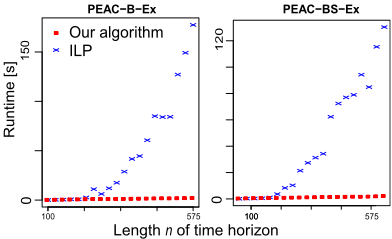
We start by comparing the performance of Algorithm 2 and Gurobi for the corresponding ILP. We simulated 20 different instances with the number of periods ranging from 100 to 600 and with a capacity of at most 1000. Figure 1 shows the average runtimes for each time horizon selected. As expected, the times for solving instances with Algorithm 2 were significantly shorter and remained consistently within seconds even for the largest simulated values of C and n, whereas Gurobi often exceeded the time limit of 180 seconds to solve them.
We also conducted simulations regarding PEAC-B-U, PEAC-BS-U, PEAC-B and PEAC-BS with 50 different lengths n of time horizons, ranging from 100 to 10000. For each time horizon considered, we simulated 100 instances and computed the average runtime. As expected from Theorem 4, the battery size had little impact on the algorithm performance. Our experiments showed that the runtime grows linearly in n in the simulated instances both for Algorithm 1 and the IP. We observe that the ILP solver performs better when there are many periods with high demands and few periods with excess energy, otherwise Algorithm 1 performed better. In both cases, the runtimes were similar to each other. We defer full results for these experiments to the full version.
Acknowledgements
Laura Codazzi was supported by the Graduate School "sharing.city.college" of ahoi.digital. Gergely Cs´aji was supported by the Hungarian Scientific Research Fund, OTKA, Grant No. K143858, by the Momentum Grant of the Hungarian Academy of Sciences, grant number 2021-1/2021 and by the Ministry of Culture and Innovation of Hungary from the National Research, Development and Innovation fund, financed under the KDP-2023 funding scheme (grant number C2258525).
@inproceedings{ijcai2024p207,
  title     = {Efficient Cost-Minimization Schemes for Electrical Energy Demand Satisfaction by Prosumers in Microgrids with Battery Storage Capabilities},
  author    = {Codazzi, Laura and Csáji, Gergely and Mnich, Matthias},
  booktitle = {Proceedings of the Thirty-Third International Joint Conference on
               Artificial Intelligence, {IJCAI-24}},
  publisher = {International Joint Conferences on Artificial Intelligence Organization},
  editor    = {Kate Larson},
  pages     = {1873--1880},
  year      = {2024},
  month     = {8},
  note      = {Main Track},
  doi       = {10.24963/ijcai.2024/207},
  url       = {https://doi.org/10.24963/ijcai.2024/207},
}
TY - CPAPER TI - Efficient Cost-Minimization Schemes for Electrical Energy Demand Satisfaction by Prosumers in Microgrids with Battery Storage Capabilities AU - Codazzi, Laura AU - Csáji, Gergely AU - Mnich, Matthias T2 - Proceedings of the Thirty-Third International Joint Conference on Artificial Intelligence, IJCAI-24 PB - International Joint Conferences on Artificial Intelligence Organization PY - 2024 SP - 1873 EP - 1880 DO - 10.24963/ijcai.2024/207 UR - https://doi.org/10.24963/ijcai.2024/207 ER -Copied
Machine-readable versions of this paper, for tools and AI agents:





