Bridging the Gap between General and Down-Closed Convex Sets in Submodular Maximization

1 Introduction

Optimization of continuous DR-submodular functions (and the strongly related discrete submodular set functions) has experienced a notable surge in significance in recent times, marking a pivotal development within the domain of nonconvex optimization. The tools developed in this context adaptively tackle challenges related to real-world applications at the forefront of various fields such as data summarization [Mualem et al., 2023; Hassani et al., 2017; Bian et al., 2019; Mitra et al., 2021; Soma and Yoshida, 2017], robotics [Shi et al., 2021; Tukan et al., 2023], and human brain mapping [Salehi et al., 2017], among many others. Most of the works in the literature focused either on DRsubmodular optimization for monotone objective functions, or subject to a down-closed convex set constraint. 1 However, real-world problems are often naturally captured as optimization of a non-monotone DR-submodular function over a constraint convex set that is not down-closed. For example, imagine an online shopping platform optimizing its product recommendations within strict interface size constraints. The challenge faced by the store involves designing concise summaries that respect upper and lower bounds on product inclusion (these bounds are imposed by the user interface, and they form a non-down-closed constraint), and are good with respect to an objective function balancing between diversity and relevance in the displayed recommendations (which naturally yields a non-monotone objective).

* A full version of this paper, including all details and proofs omitted here, is available in [Mualem et al., 2024].

Motivated by scenarios similar to the one given above, and optimization under fairness constraints [El Halabi et al., 2023; Halabi et al., 2023; Yuan and Tang, 2023], some recent works have delved into the maximization of nonmonotone DR-submodular functions over general (not necessarily down-closed) convex set constraints. Unfortunately, in general, no constant approximation can be obtained for this problem in sub-exponential time due to a hardness result by Vondr´ak [2013]. However, Durr et al. [2021] observed that Vondr´ak's proof of the hardness result was based on a class of instances whose convex sets K include no point whose ℓ∞- norm is less than 1. 2 In light of this observation, Durr et al. [2021] considered a parametrization of the problem based on the minimum ℓ∞ norm of any vector in K (this minimum is usually denoted by m), and were able to provide a subexponential time 1 3√3 (1-m)-approximation for the problem of optimizing a non-monotone DR-submodular function subject to a general convex set K.

The work Durr et al. [2021] has inspired a new line of research. Th´˘ang & Srivastav [2021] showed how to obtain a similar result in an online (regret minimization) setting, and Du et al. [2022] improved the approximation ratio in the offline setting to 14 (1 - m) (while still using sub-exponential time). More recently, the first polynomial time algorithm for the problem, guaranteeing the same approximation ratio as [Du et al., 2022], has been provided by Du [2022]; and subsequently, Mualem & Feldman [2023] obtained the same result in the online setting. In their work, Mualem & Feldman also proved a hardness result, showing that 1 4 (1 - m)- approximation is the best approximation ratio that can be obtained in sub-exponential time, which shows that the last algorithms are optimal, and settles the approximability of the problemwith respect to this parametrization.

1 A set K is down-closed with respect to a domain X if, for every two vectors x, y ∈ X , x ∈ K whenever y ∈ K and y coordinatewise dominates x. As is standard, we usually omit the domain when talking about down-closed sets, and implicitly assume it to be the domain of the objective function.

2 For simplicity, we implicitly assume that the domain of the objective function and the convex set constraint is [0, 1]n . This assumption is without loss of generality (see Section 2).

Our contribution. Every down-closed convex body has m = 0. The reverse is not true, but one could hope that convex bodies having m = 0 admit as good approximation as down-closed convex bodies. Unfortunately, the hardness result of Mualem & Feldman disproves this hope since the state-of-the-art approximation ratio for down-closed bodies is 0.401 [Buchbinder and Feldman, 2023]. This prompts the question of whether there is a different way to look at the problem (beyond parametrization by m) that will provide a smooth interpolation between the approximability obtainable for down-closed and general convex bodies. In this work, we suggest such an interpolation based on a decomposition of the convex body constraint into two distinct convex bodies: a down-closed convex body and a general convex body. Our key results based on this decomposition are as follows.

• We provide a novel polynomial time (offline) algorithm for maximizing DR-submodular functions over convex sets given as a composition of a down-closed convex body KD and a general convex body KN. Our algorithm always recovers at least the 14 (1-m)-approximation of Du [2022]. The approximation guarantee smoothly improves when a significant fraction of the value of the optimal solution belongs to the down-closed part KD of the decomposition. In particular, when the convex body happens to be entirely down-closed, our algorithm guarantees e-1 ≈ 0.367-approximation, which recovers the approximation ratio for down-closed convex bodies obtained by the Measured Continuous Greedy technique [Bian et al., 2017a; Feldman et al., 2011]. 3
• We provide a novel online (regret minimization) algorithm for the same problem that replicates the guarantees of our offline algorithm, up to a regret term that is proportional to the square root of the number of time steps.
• We demonstrate that a decomposition of the kind that we use can be naturally obtained for various machinelearning applications, and use this fact to empirically demonstrate the superiority of our proposed algorithms compared to existing methods across various offline and online applications, namely, offline and online rev-

3 As mentioned above, the state-of-the-art approximation ratio for down-closed convex body constraints is 0.401. However, all current algorithms for such convex bodies with ratios better than e-1 are based on the Measured Continuous Greedy technique (with additional, often impractical, components). To keep our algorithms simple and our message clear, we only aim to recover e-1 - approximation for down-closed convex bodies.

enue maximization, quadratic programming and location summarization. In the full version of this paper [Mualem et al., 2024], we also provide theoretical implications for fairness settings.

1.1 RelatedWork

DR-submodular maximization has recently emerged as a key tool in numerous applications within the realms of machine learning and statistics. This surge in relevance has prompted a growing number of studies in this field. In what follows, we provide a brief overview of the main results in this field.

OfflineDR-submodular optimization. The study of maximization of DR-submodular functions over down-closed convex sets was initiated by Bian et al. [2017a]. Their work showcased the effectiveness of a modified Frank-Wolfe algorithm, grounded in the greedy method introduced by [Calinescu et al., 2011] in the context of set functions, ensuring (1 - 1/e)-approximation for the problem when the objective function is guaranteed to be monotone (this is optimal due to [Nemhauser and Wolsey, 1978]). Hassani et al. [2017] subsequently identified a limitation in the algorithm proposed by [Bian et al., 2017a], revealing its lack of robustness in stochastic settings where only an unbiased estimator of the gradient is available. To mitigate this limitation, Hassani et al. [2017] demonstrated that gradient methods exhibit robustness in such scenarios, achieving 1/2-approximation.

When the DR-submodular function is not guaranteed to be monotone, the approximation task becomes notably more challenging. In separate works, Bian et al. [2019] and Niazadeh et al. [2020] introduced distinct algorithms, both ensuring 1/2-approximation for the maximization of nonmonotone DR-submodular functions over a hypercube constraint, which is the best possible [Feige et al., 2011]. It is noteworthy that (one version of) the algorithm proposed by [Niazadeh et al., 2020] applies also to (non-DR) submodular functions. As mentioned above, the state-of-the-art approximation for maximizing non-monotone DR-submdoular functions subject to a down-closed convex body constraint is 0.401 [Buchbinder and Feldman, 2023].

Recently, Pedramfar et al. [2023] introduced a unified approach for maximization of continuous DR-submodular functions that encompasses a range of settings and oracle access types, while Mualem & Feldman [2022] suggested a parameter termed monotonicity-ratio allowing for a smooth interpolation between e-1 -approximation for non-monotone objectives and (1 - 1/e)-approximation for monotone objectives.

Online (regret minimization) DR-submodular optimization. Chen et al. [2018] were the first to address online maximization of monotone DR-submodular functions over a convex set (for monotone objective functions the distinction between down-closed and general convex sets is irrelevant). They introduced two algorithms: one ensuring (1 - 1/e)- approximation with approximately O(√T)-regret, and another algorithm that is resilient to stochastic settings, but guarantees only 1/2-approximation up to the same regret. Later, Chen et al. [2019] proposed an algorithm that combines (1 - 1/e)-approximation with roughly O(√T )-regret and robustness, and Zhang et al. [2019] demonstrated how to reduce the number of gradient calculations per time step to one at the expense of increasing the regret to roughly O(T 4/5 ). The last reduction is particularly relevant for bandit versions of the problem (we refer the reader to [Pedramfar et al., 2023] for a detailed overview of such versions).

For online optimization of DR-submodular functions that are not guaranteed to be monotone, Th´˘ang & Srivastav [2021] introduced three algorithms. One of these algorithms is applicable to general convex set constraints, and was later improved over by Mualem and Feldman [2023], as discussed above. Another was designed for maximization over the entire hypercube, achieving 1/2-approximation with approximately O(√T )-regret. The last algorithm of [Th´˘ang and Srivastav, 2021] addresses down-closed convex set constraints, and attains e-1 -approximation with roughly O(T 2/3 )-regret.

1.2 Paper Organization

In Section 2, we formally describe the problem we consider. Then, in Section 3, we discuss the technique underlying our results. Our offline and online algorithms, which are based on this technique, can be found in Sections 4 and 5, respectively. Finally, Section 6 compares the empirical performance of our algorithms on multiple machine learning applications with the performance of previously suggested algorithms from the literature.

2 Preliminaries

In this section, we formally present the problem we consider in this paper and the notation that we use. Let us begin with the definition of DR-submodular functions, which are continuous analogs of submodular set functions first defined by Bian et al. [2017b]. Formally, given a domain X = ∏ni=1 Xi, where Xi is a closed range in R for every i ∈ [n], a function F : X → R is called DR-submodular if the inequality

holds for every two vectors a, b ∈ X, positive value k and coordinate i ∈ [n] obeying a ≤ b and b + kei ∈ X (here and throughout the paper, ei denotes the standard i-th basis vector, and comparison between two vectors should be understood to hold coordinate-wise). Bian et al. [2017b] observed that for continuously differentiable functions F, the above definition of DR-submodulrity is equivalent to

and for twice differentiable functions F , it is equivalent to the Hessian being non-positive at every vector x ∈ X .

In this work, we study the problem of maximizing a nonnegative DR-submodular function F : X → R≥0 subject to a convex body K ⊆ X constraint. We are interested in the approximation guarantee that can be obtained for this problem based on a particular decomposition of K into two other convex bodies: a convex body KD that is down-closed with respect to X and a (not necessary down-closed) convex body KN. Formally, by saying that KD and KN are a decomposition of K, we mean that K = (KN + KD) ∩ X, where KN + KD ≜ {y + z | y ∈ KN, z ∈ KD}.

For simplicity, we assume (throughout the paper) that the domain X of our objective functions is [0, 1]n . This assumption is without loss of generality since there is a natural linear mapping from X to [0, 1]n preserving the above discussed properties of F and K. Additionally, as is standard in the field, we assume that F is β-smooth for some β > 0. A function F : [0, 1]n → R is call β-smooth if it is continuously differentiable, and obeys

Another standard assumption in the field is that the relevant convex-bodies (KN and KD in our case) are solvable, i.e., that one can efficiently optimize linear functions over them. We take a step further, and assume the ability to optimize linear functions over any convex body defined by the intersection of a polynomial number of linear constraints and constraints requiring particular vectors to belong either to KN or to KD. This assumption appeared (often implicitly) in many previous works (see, for example, [Buchbinder and Feldman, 2023; Ene and Nguyen, 2016; Mualem and Feldman, 2023]), and is theoretically justified by the well-known equivalence between separability and solvability.

We often refer below to the diameter D of K. This diameter is defined as D ≜ maxx,y∈K ∥x - y∥2.

2.1 Additional Vector Operations

Following Buchbinder and Feldman [2023], we use the following coordinate-wise vector operations. To reduce the number of parentheses necessary, we assume that both these operations have a higher precedence compared to vector addition and subtraction.

Definition 2.1. Given two vectors x, y ∈ [0, 1]n ,

• we denote by x⊙y their coordinate-wise multiplication (also known as the Hadamard product).
• we denote by x ⊕ y their coordinate-wise probabilistic sum. In other words, for every i ∈ [n], (x ⊕ y)i ≜ xi + yi - xiyi = 1 - (1 - xi)(1 - yi).

As was noted by [Buchbinder and Feldman, 2023], the operation ⊕ is symmetric and associative. We also use ¯0 and ¯1 to represent the all-zeros and all-ones vectors, respectively.

2.2 Online Optimization

In the online (regret minimization) version of the problem we consider in this work, there are L time steps. 4 In every time step ℓ ∈ [L], the adversary selects a non-negative β-smooth DR-submodular function Ft, and then the algorithm should select a distribution Pℓ of points in K = (KN + KD) ∩ [0, 1]n without knowing Ft (the function Ft is revealed to the algorithm only after Pℓ is selected). The objective of the algorithm is to maximize ∑Lℓ=1 Ex∼Pℓ [Fℓ(x)], and its success in doing so is measured compared to the best fixed solution (i.e., any two vectors oN ∈ KN and oD ∈ KD such that oN + oD ∈ [0, 1]n ).

4 The number of time steps is usually denoted by T in the literature. However, we use L in this paper to avoid confusion with the parameter T traditionally used by continuous submodular maximization algorithms (including our own algorithms).

Let us elaborate a bit on the last point. If the functions F1, F2, . . . , FL were all known upfront, one could execute the offline algorithm we develop to get a set of solutions x(1) , x(2) , . . . , x(L) such that ∑Lℓ=1 Fℓ(x(ℓ) ) ≥ ψ(∑Lℓ=1 Fℓ(oN + oD), ∑Lℓ=1 Fℓ(oD)) for some function ψ (the structure of the function ψ is determined by the guarantee of Theorem 4.1 below). Since an online algorithm has to select the output distribution Pℓ before seeing the function Fℓ, it can only guarantee

for some regret function R(L). Asymptotically, for our online algorithm, R(L) grows proportionally to √L, and therefore, for large L values, the average guarantee of our online algorithm per function Fℓ approaches the one of our offline algorithm. As usual for online settings, we assume that the range of the functions F1, F2, . . . , FL is [0, 1].

3 Our Technique

Our algorithms maintain vectors y ∈ KN and z ∈ KD. Intuitively, the vector y is maintained by the Frank-Wolfe variant developed by Mualem and Feldman [2023] for nondown-closed polytopes, and the vector z is maintained by the continuous-greedy-like variant of Frank-Wolfe developed by Bian [2017a] for down-closed polytopes. Combining the two algorithms requires us to solve some technical issues. For example, it is necessary to run the two algorithms in parallel since they both depend on the coordinates of the solution growing at a bounded rate, and it is necessary to create a correlation between the algorithms to guarantee that y + z remains within [0, 1]n . However, it turns out that the more interesting question is regarding the best way to combine the two vectors y and z into the output solution of the algorithm.

The most natural approach is to consider the sum y + z as the output solution. Unfortunately, this does not work well since it results in coordinates of the solution growing too fast. To make this more concrete, we note that our algorithms, as well as the algorithms of [Bian et al., 2017a] and [Mualem and Feldman, 2023], simulate continuous algorithms working from time t = 0 until time t = 1. Consider now a particular coordinate j ∈ [n]. Up until time t ∈ [0, 1], our algorithms spend (up to) t units of "energy" on this coordinate. A fraction x ∈ [0, t] of this "energy" is invested in growing yj, and the remaining t - x "energy" is invested in growing zj. By the properties of the algorithms of [Bian et al., 2017a] and [Mualem and Feldman, 2023], this investment of "energy" leads to yi = 1 - e-x and zi = 1-ex-t , which in the worst case can make (y+z)i as large as 2(1 - e-t/2 ). To get a better upper bound on the coordinates of the solution, we have to use y ⊕ z as the output solution. Note that this choice guarantees that (y⊕z)j ≤ 1- [1-(1-e-x )] · [1-(1-ex-t )] = 1-e-t , which is always better (for t > 0) compared to the bound of 2(1 - e-t/2 ) obtained above.

While the use of y ⊕ z is useful, it does not come without a cost. As mentioned above, our algorithms simulate continuous algorithms, which is a common practice in the literature about submodular maximization. To discretize these algorithms, one has to split time into steps, and then do in each step a single modification of the vectors y and z simulating all the modifications done by the continuous algorithm throughout the step. The standard way in which this is done is as follows. Assume that, at the beginning of the step, the continuous algorithm increases y at a rate of y′ and z at a rate of z′ , then the discrete algorithm should increase y by εy′ and z by εz′ , where ε is the size of the step. Unfortunately, this standard practice results in y ⊕ z changing by εy′ ⊙(¯1-z)+εz′ ⊙(¯1-y)-ε2 · (y′ ⊙z′ ). To see why this is problematic, note that in the continuous algorithm, when y and z increase at rates of y′ and z′ , respectively, y ⊕ z increases at a rate of y′ ⊙ (¯1 - z) + z′ ⊙ (¯1 - y). Thus, the term -ε2 · (y′ ⊙ z′ ) from the previous expression represents a new kind of discretization error that we need to handle.

Another hurdle worth mentioning is that the vectors y and z are updated using two different update rules inherited from the algorithms of [Bian et al., 2017a] and [Mualem and Feldman, 2023], and the interaction between these update rules results in a guarantee on the output of the algorithm that depends also on the value of F(z). Thus, it is necessary to make sure that our algorithms maintain z in a way that also guarantees that F(z) has a good value. In the first version of our offline algorithm, we do that by assuming that we know the value v of the part of the optimal solution that belongs to KD. This knowledge allows us to force the algorithm to increase z in a way guaranteed to make F(z) competitive with v. In the other versions of our offline algorithm and in our online algorithm, we use a potential function argument to avoid the need to know v. This potential function argument is similar to an argument used by Feldman [2021] in a different submodular maximization setting.

4 Offline Maximization

In this section, we present and analyze our offline algorithm, whose guarantee is given by the next theorem.

Theorem 4.1. Let KN ⊆ [0, 1]n be a general solvable convex set, KD ⊆ [0, 1]n be a down-closed solvable convex set, and F : [0, 1]n → R≥0 be a non-negative β-smooth DRsubmodular function. Then, there exists a polynomial time algorithm that, given an error parameter ε ∈ (0, 1), outputs vectors w ∈ (KN + KD) ∩ [0, 1]n such that

where m = minx∈KN ∥x∥∞, D is the diameter of (KN+KD)∩ [0, 1]n , oN ∈ KN and o(1) D ∈ KD are any vectors whose sum belongs to (KN+KD)∩[0, 1]n , and o(2) D is any vector inKD. 5

5 The vectors o(1) D and o(2) D can be identical.

It is interesting to note that Theorem 4.1 recovers two guarantees of previous works. Specifically, by setting T = 1, ts = 0 and KN = {¯0}, the theorem implies e-1 -approximation for maximizing a DR-submodular function subject to a downclosed polytope KD, recovering the result of [Bian et al., 2017a]. Similarly, by setting T = ts = ln2 and KD = {¯0}, Theorem 4.1 implies 1/4(1-m)-approximation for maximizing a DR-submodular function subject to a general polytope KN, recovering the result of [Mualem and Feldman, 2023].

For ease of the presentation, we have three versions of our offline algorithm. The first version, appearing below as Algorithm 1, proves Theorem 4.1 under the assumption that F (o(1) D ) is known. In the full version of this paper [Mualem et al., 2024], we present the two other versions of our offline algorithm that prove Theorem 4.1 without making this assumption. One version is theoretically natural, and is the base for our online algorithm described in Section 5. However, to get the best results in practice, it is natural to make some modifications to this natural version (including ones motivated by the work of [Bian et al., 2017a]), which do not improve the theoretical guarantee of the algorithm and cannot be extended to the online version of the algorithm. Both the natural and the modified version of our algorithm are studied in the offline experiments described in Section 6.

Recall that Algorithm 1 proves Theorem 4.1 under the assumption that F(o(1) D ) is known. In its description, we assume for simplicity that ε-1 is integral. If this is not the case, ε can be replaced with ⌈ε-1 ⌉-1 , which is smaller than ε by at most a factor of 2.

Algorithm1 Frank-Wolfe/Continuous-Greedy Hybrid for Known F(o(1) D )

• 1: Let y(0) ← argminx∈KN ∥x∥∞ and z(0) ← ¯0.
• 2: for i = 1 to ε-1 do
• 3: Solve the following linear program:

• 6: end for
• 7: Return a vector maximizing F among all the vectors in {y(i) ⊕z(i) | i ∈ Z, 0 ≤ i ≤ ε-1 }.

5 Online Maximization

In this section, we consider the online (regret minimization) setting described in Section 2.2. The algorithm we present and analyze has the guarantee given by the next theorem.

Theorem 5.1. Let KN ⊆ [0, 1]n be a general solvable convex set, and KD ⊆ [0, 1]n be a down-closed solvable convex set. If the adversary chooses only non-negative β-smoothDRsubmodular functions Fℓ : [0, 1]n → [0, 1], then there exists a polynomial time online algorithm that, given value ε ∈ (0, 1), outputs at every time step ℓ ∈ [L] a distribution Pℓ over vectors in (KN + KD) ∩ [0, 1]n guaranteeing that

where m = minx∈KN ∥x∥∞, D is the diameter of (KN + KD) ∩ [0, 1]n , G = max{maxx∈(KN+KD)∩[0,1]n ∥∇Ft(x)∥2, maxx∈KD ∥∇Ft(x)∥2, }, and oN ∈ KN and oD ∈ KD are any vectors whose sum belongs to (KN + KD) ∩ [0, 1]n .

Note the following two remarks about Theorem 5.1.

• Section 2.2 states that the regret of our online algorithm (compared to the offline algorithm) asymptotically grows as √L. This might seem to contradict the presence of the error term O(εβLD2 ) in the guarantee of Theorem 5.1. However, this is not the case since this error term is part of the ψ functions mentioned in Section 2.2 (because the term O( εβD2 1-m ) appears in the guarantee of Theorem 4.1).
• Theorem 4.1 considers two vectors o(1) D , o(2) D ∈ KD. A similar result could be proved in Theorem 5.1. However, in the online setting, the algorithm is required to be competitive against any fixed solution. Thus, we felt that it is more natural to state Theorem 5.1 for the case in which o(1) D and o(2) D are the same vector (denoted by oD).

The central component in the proof of Theorem 5.1 is the following proposition, which is a variant of Theorem 5.1 in which (i) ts is a parameter of the algorithm, and (ii) the algorithm outputs in each time step a single vector rather than a distribution over vectors.

Proposition 5.2. Let KN ⊆ [0, 1]n be a general solvable convex set, and KD ⊆ [0, 1]n be a down-closed solvable convex set. If the adversary chooses only non-negative β-smoothDRsubmodular functions Fℓ : [0, 1]n → [0, 1], then there exists a polynomial time online algorithm that, given parameters ts ∈ [0, 1] and ε ∈ (0, 1), outputs at every time step ℓ ∈ [L] a vector w(ℓ) ∈ (KN + KD) ∩ [0, 1]n guaranteeing that

where m = minx∈KN ∥x∥∞, D is the diameter of (KN + KD) ∩ [0, 1]n , G = max{maxx∈(KN+KD)∩[0,1]n ∥∇Ft(x)∥2, maxx∈KD ∥∇Ft(x)∥2}, and oN ∈ KN and oD ∈ KD are any vectors whose sum belongs to (KN + KD) ∩ [0, 1]n .

Algorithm 2 Online Frank-Wolfe/Continuous -Greedy Hybrid

• 1: for i = 1 to ε-1 do
• 2: Initialize an instance Ei of Regularized-Follow-theLeader for the convex body {(a, b) | a ∈ KN, b ∈ KD, a + b ∈ [0, 1]n }.
• 3: end for
• 4: Let m←minx∈KN ∥x∥∞.
• 5: for ℓ = 1 to L do
• 6: Let y(0,ℓ) ← argminx∈KN ∥x∥∞, z(0,ℓ) ← ¯0.
• 7: for i = 1 to ε-1 ts do
• 8: Let (a(i,ℓ) , b(i,ℓ) ) be the vector picked by Ei in time step ℓ.
• 9: Let y(i,ℓ) ← (1 - ε) · y(i-1,ℓ) + ε · a(i,ℓ) .
• 10: Let z(i,ℓ) ← z(i-1,ℓ) + ε · (1 - z(i-1,ℓ) ) ⊙ b(i,ℓ) .
• 11: end for
• 12: for i = ε-1 ts + 1 to ε-1 do
• 13: Let a(i,ℓ) ← y(i-1,ℓ) .
• 14: Let b(i,ℓ) be a vector consisting of the last n coordinates of the vector picked by Ei in time step ℓ.
• 15: Let y(i,ℓ) ← y(i-1,ℓ) .

• 17: end for
• 18: Set the vector y(ε-1 ,ℓ) ⊕z(ε-1 ,ℓ) as the output for time step ℓ.
• 19: for i = 1 to ε-1 ts do
• 20: Let g(i,ℓ) be the vector in R2n obtained as follows. The first n coordinates of this vector are given by e2εi∇Fℓ(y(i-1,ℓ) ⊕ z(i-1,ℓ) ) ⊙ (¯1 - z(i-1,ℓ) ), and the other n coordinates of g(i,ℓ) are equal to e2εi∇Fℓ(y(i-1,ℓ) ⊕ z(i-1,ℓ) ) ⊙ (¯1 - z(i-1,ℓ) ) ⊙ (¯1-y(i-1,ℓ) )+(1-m)·eεi (ts-εi)·∇Fℓ(z(i-1,ℓ) )⊙ (1 - z(i-1,ℓ) ).
• 21: Pass g(i,ℓ) as the adversarially chosen vector d(ℓ) for Ei.
• 22: end for
• 23: for i = ε-1 ts + 1 to ε-1 do
• 24: Let g(i,ℓ) be a vector in R2n obtained as follows. The first n coordinates of this vector are all zeros, and the other n coordinates of g(i,ℓ) are equal to ∇Fℓ(y(i-1,ℓ) ⊕ z(i-1,ℓ) ) ⊙ (¯1 - z(i-1,ℓ) ) ⊙ (¯1 - y(i-1,ℓ) ).
• 25: Pass g(i,ℓ) as the adversarially chosen vector d(ℓ) for Ei.
• 26: end for
• 27: end for

Let us explain why Proposition 5.2 implies Theorem 5.1. The guarantee given in Theorem 5.1 remains unchanged (up to the constants hidden by the big O notation) if the maximum over ts ∈ [0, 1] is restricted to the set of O(ε-1 ) values that are integer multiples of ε between 0 and 1. If we knew upfront what value from this set leads to the best guarantee for Proposition 5.2, then we could use the algorithm of this proposition to get the guarantee of Theorem 5.1.

Unfortunately, in reality, we do not usually know upfront the best value for ts. Nevertheless, since there are only O(ε-1 ) such values that need to be considered, we can use a regret minimization algorithm (such as the one of [CesaBianchi et al., 2007]) to get in each time step a distribution over solutions whose expected value is at least as good as the guarantee of Proposition 5.2 for the best value of ts, up to an error term of O(√Llnε-1 ). Thus, Theorem 5.1 indeed follows from Proposition 5.2.

At this point, we would like to describe the algorithm that we use to prove Proposition 5.2, which is given as Algorithm 2. Similarly to the Meta-Frank-Wolfe algorithm of [Chen et al., 2018], Algorithm 2 uses multiple instances of an online algorithm for linear optimization. Specifically, we use the algorithm Regularized-Follow-the-Leader due to [Abernethy et al., 2008], which has the following behavior. There are L time steps. In every time step ℓ ∈ [L], the algorithm selects a vector u(ℓ) ∈ K for some given convex body K, and then an adversary reveals to the algorithm a vector d(ℓ) that was chosen independently of u(ℓ) . RegularizedFollow-the-Leader guarantees that

where G′ = max1≤ℓ≤L ∥d(ℓ) ∥2 and D′ is the diameter of K. Algorithm 2 follows the same general structure of our offline algorithm, with two main modifications: the linear programs of the offline algorithm are replaced by instances of the online linear optimization algorithm that we use, and the vector corresponding to i = T -1 is used as the output instead of the best vector among multiple options.

In the pseudocode of Algorithm 2, we implicitly assume that ε ≤ 1/70 and εts is integral. The first assumption is without loss of generality since we can decrease ε to be 1/70 if its original value is larger, and the second assumption is without loss of generality because the coefficients in the guarantee of Proposition 5.2 change only by O(ε) when ts is modified by up to ε to make tsε integral.

6 Applications and Experimental Results

In this work, we study the empirical performance of the offline and online algorithms described in the previous sections on three machine learning tasks. We present one application here, and defer the rest to the full version of this paper [Mualem et al., 2024]. The full version also includes empirical stability and ablation studies of our offline algorithm.

6.1 Revenue Maximization

As our first experimental setting, we consider the following revenue maximization setting, which was also considered by [Mualem and Feldman, 2023; Soma and Yoshida, 2017; Th´˘ang and Srivastav, 2021]. The objective of some company is to promote a product to users to boost revenue through the "word-of-mouth" effect. The problem of optimizing this objective can be formalized as follows. The input is a weighted undirected graph G = (V, E) representing a social network, where wij represents the weight of the edge between vertex i and vertex j (with wij = 0 if the edge (i, j) is absent from the graph). If the company allocates a cost of xi units to a user i ∈ V , then that user becomes an advocate of the product with a probability of 1 - (1 - p)xi , where p ∈ (0, 1) is a parameter. Note that this formula implies that each ε unit of cost invested in the user independently contributes to the chance of making the user an advocate. Furthermore, by investing a full unit in the user, the user becomes an advocate with a probability of p [Soma and Yoshida, 2017].

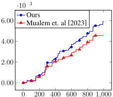
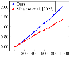
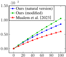
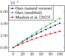
Figure 1: Results of the revenue maximization experiments. In each plot, the x-axis is the timestep, and the y-axis is the corresponding function value.

Given a set S ⊆ V of users who have become advocates for the product, the expected revenue is related to the total influence of the users in S on non-advocate users, which is formally expressed as ∑i∈S ∑j∈V \S wij . Hence, the objective function F : [0, 1]V → R≥0 in this setting is defined as the expectation of the aforementioned expression, i.e.,

It has been demonstrated that F is a non-monotone DRsubmodular function [Soma and Yoshida, 2017].

We conducted experiments in both online and offline scenarios based on instances of the aforementioned setting derived from two distinct datasets. The first dataset is sourced from a Facebook network [Viswanath et al., 2009], encompassing 64K users (vertices) and 1M unweighted relationships (edges). The second dataset is based on the Advogato network [Massa et al., 2009], comprising 6.5K users (vertices) and 61K weighted relationships (edges).

Online Setting. In our online experiments, inspired by [Mualem and Feldman, 2023], we set the number of time steps to L = 1000, with p = 0.0001. At each time step ℓ, the objective function is defined by selecting a uniformly random subset Vℓ ⊆ V of a given size, and then retaining only edges connecting two vertices of Vℓ. For the Advogato network, Vℓ is of size 200, and for the larger Facebook network, Vℓ is of size 15,000. The above objective functions are optimized subject to the constraint 0.1 ≤ ∑i xi ≤ 1, which represents both minimum and maximum investment requirements. Notably, the intersection of this constraint with the implicit box constraint forms a non-down-monotone feasibility polytope. However, this polytope can be decomposed into two polytopes: (i) KN, a polytope defined by the equality

∑ni=1 xi = 0.1, and (ii) KD, a down-closed polytope defined by ∑ni=1 xi ≤ 0.9. Observe that (KD+KN)∩[0, 1]n is indeed the original polytope, and thus, this is a valid decomposition of this polytope.

In our experiments, we have compared the performance of our algorithm from Section 5 with the online algorithm of Mualem & Feldman [2023], which is the current state-of-theart algorithm for the online setting. In both algorithms, we have set the number of online linear optimizers used to be 100 (which corresponding to setting the error parameter ε to 0.01 in our algorithm and to ln2/100 in the algorithm of Mualem & Feldman). The results of our experiments on the Advogato and Facebook networks can be found in Figures 1a and 1b, respectively. In both experiments, our algorithm significantly outperforms the state-of-the-art algorithm.

Offline Setting. Our offline experiments are similar to their online counterparts. However, since there is only one objective function in this setting, we run the experiment on the entire network graph. In this setting, we compared our offline algorithm (see Section 4 for a discussion of the versions of this algorithm used in the experiments) with the current state-of-the-art algorithm from [Mualem and Feldman, 2023] (which is an explicit version of the algorithm of Du [2022]). Both algorithms have been executed for T = 100 iterations, and the error parameter ε was set accordingly (which again means 0.01 in our algorithm and ln2/100 in the algorithm of Mualem & Feldman). The results of the offline experiments on the Advogato and Facebook networks can be found in Figures 1c and 1d, respectively. One can observe that our method consistently outperforms the previous state-of-the-art.

7 Conclusion

We have presented novel offline and online algorithms for DR-submodular maximization subject to a general convex body constraint. Our algorithms are able to provide a smooth interpolation between the approximability of general and down-closed convex bodies by considering a decomposition of the convex body constraint into a down-closed convex body and a general convex body. In addition to giving a theoretical analysis of our algorithms, we have demonstrated their empirical superiority (compared to state-of-the-art methods) in various online and offline machine learning applications.

Acknowledgements

The work of Loay Mualem and Moran Feldman has been partially supported by Israel Science Foundation (ISF) grant number 459/20.