Real-World Networks Are Low-Dimensional: Theoretical and Practical Assessment

1 Introduction

A key technique for understanding and analyzing large complex data sets is to embed them into a low-dimensional geometric space. Hence, the search for embedding and dimensionality reduction algorithms has become an important direction in data analysis and artificial intelligence research [Sarveniazi, 2014; Camastra and Staiano, 2016; Nickel and Kiela, 2017]. Embedding algorithms commonly require a metric that captures the similarities between data points, which is often abstracted using a graph whose vertices represent the data points and two vertices are connected if they are close with respect to this metric. The algorithm then determines geometric positions for these vertices such that connected vertices are close together. Such approaches often require an a-priori knowledge of the dimensionality, which is unknown in most applications. Heuristic approaches try to determine the dimensionality of a dataset by embedding it in spaces of different dimensionality and choosing the value that yields the optimal embedding [Levina and Bickel, 2004; Yin and Shen, 2018; Gu et al., 2021].

∗The full version which includes all proofs can be found at https: //arxiv.org/abs/2302.06357.

The recent work of [Almagro et al., 2022] gives a new algorithm for learning the dimensionality that does not require embeddings. Instead, given a graph as input, their method counts the number of short - i.e. length 3, 4 and 5 - cycles of a graph. It then generates a search space consisting of random graphs that are generated from a geometric model of varying parameters, including the dimensionality of the space. Finally, a data-driven classifier finds the random graph of the search space that resembles the input graph the most and returns its dimensionality. A remarkable observation, that comes from using their algorithm to learn the dimensionality of real-world networks, is that the vast majority of networks has very low dimensionality, which is independent of the size of the network.

A downside of the aforementioned approach is that it relies on machine learning techniques that are computationally heavy with no asymptotic run-time guarantees and lacks theoretical explanation for its solution quality. In order to argue with mathematical rigour, one requires to work with welldefined mathematical objects. A common approach to incorporate such an object is that of average-case analysis, that is, assume that the input graph comes from a well-defined random graph model. The random graph model that has been mostly considered so far in the literature is that of spherical random graphs, where vertices are generated independently and uniformly at random as points on the surface of a ddimensional sphere and two vertices are connected if their angle is bellow a certain threshold. It can be easily shown that, as the number of dimensions increases, spherical random graphs converge to Erd˝os-R´enyi graphs, the classical random graph model where edges are drawn independently. A series of works considers the statistical testing problem of detecting whether a given graph is a spherical random graph or an Erd˝os-R´enyi graph and determines the parameter regime under which this can be done [Devroye et al., 2011; Bubeck et al., 2016; Brennan et al., 2020; Liu and R´acz, 2023b; Liu et al., 2022]. Follow-up works consider noisy settings [Liu and R´acz, 2023a] or anisotropic geometric random graphs [Eldan and Mikulincer, 2020; Brennan et al., 2024], where each dimension has a different influence on the drawing of edges. The techniques of the aforementioned results can also be used for determining the dimensionality of the given graph [Bubeck et al., 2016, Theorem 5].

A characteristic of the random graph models considered in the aforementioned works, i.e. spherical random graphs and Erd˝os-R´enyi graphs, is that the degree distributions of the generated graphs is concentrated around its expected value; this contrasts the power-law degree distributions observed in real-world networks [Faloutsos et al., 1999]. While a latent geometric space appears to be a fundamental requirement for a random graph model that captures the high clustering coefficient [Krioukov, 2016; Boguna et al., 2021] and small diameter [Friedrich et al., 2013] observed in real-world networks, one needs to also consider the heterogeneity observed in the vertex degrees. A popular model in network theory capturing all previous properties is based on generating points on the hyperbolic plane instead of Euclidean space [Boguna et al., 2010]. However, it is not clear what the non-geometric counterpart to test against is in this case.

Our Contribution. In this article we bring theory and practice closer together and provide a mathematical explanation for the very low dimensionality of real-world networks that has been observed in practice [Almagro et al., 2022]. To this end, we build our analysis on Geoemtric inhomogeneous random graphs (GIRGs), a model which was recently shown to capture many quantifiable properties of real-world networks [Bl¨asius and Fischbeck, 2022]. Our rigorous proofs give new insights about the model with which we are able to design a linear-time algorithm for learning the dimensionality of a network and show that when the input is a GIRG our algorithm returns the correct answer with high probability. We note that the small running time is an important advantage compared to the previously mentioned methods, as it enables working with the increasingly large networks that we encounter in practice.

2 Preliminaries

We use standard Landau notation to describe the asymptotic behavior of functions for sufficiently large n. That is, for functions f, g, we write f(n) = O(g(n)) if there is a constant c > 0 such that for all sufficiently large n, f(n) ≤ cg(n). Similarly, we write f(n) = Ω(g(n)) if f(n) ≥ cg(n) for sufficiently large n. If both statements are true, we write f(n) = Θ(g(n)). Regarding our study of the clustering coefficient, some results make a statement about the asymptotic behavior of a function with respect to a sufficiently large d. These are marked by Od(·), Ωd(·), Θd(·), respectively.

Geometric Inhomogeneous Random Graphs & ChungLu Graphs. Geometric inhomogeneous random graphs (GIRGs) as introduced in [Bringmann et al., 2017] are defined as follows. Let G(n, d, β,w0, λ) = (V,E) denote the n-vertex graph obtained in the following way. For each v ∈ V , we independently sample a weight wv from the Pareto distribution P with parameters 1 - β and w0, and we draw a position xv uniformly on the d-dimensional torus. Then, edges are formed depending on the weights of the vertices, the distances between the corresponding positions, and the constant λ > 0.

More precisely, the distribution of the weights is described by the distribution function

where wmin > 0 and β > 2 are assumed to be constants, the constraint on the latter ensuring that that a single weight has finite expectation (and thus the average degree in the graph is constant), but possibly infinite variance. The density of wv is ρwv (x) = (β - 1/w1-β 0 )x-β . We denote the sequence of the drawn weights by {w}n1 .

The position xv in the d-dimensional torus Td is drawn uniformly at random according to the standard Lebesgue measure. We denote the i-th component of xv by xvi. Distances on the torus are then measured using the Lp-norm for a constant 1 ≤ p ≤ ∞. That is, we define

Note that L∞ is a natural metric on the torus as B∞(r), the ball of radius r under this norm, is a cube and "fits" entirely into Td for all 0 ≤ r ≤ 1.

Given the weights and positions, two vertices u and v are adjacent if and only if their distance ∥xu - xv∥p is at most the connection threshold tuv, which is defined such that the marginal connection probability of u, v is

for κuv = min{n, λwuwv}. Under L∞-norm, and for µ = 2d /λ, this connection threshold is

The GIRG model has a natural non-geometric counterpart where the weight distribution of the vertices is the same as in GIRGs but the edges are now sampled independently, with probability

This inhomogeneous random graph model is known as the Chung-Lu random graph model and has been extensively studied in literature [Aiello et al., 2001; Chung and Lu, 2002a; Chung and Lu, 2002b].

Hence for our analysis, we are now equipped with an appropriate geometric random graph model and its nongeometric variant. Note that the two models converge as the number of dimensions in the GIRG model goes to infinity, i.e., the total variation distance of the two models goes to zero, as it was shown in [Friedrich et al., 2023a, Theorem 1]. Finally, let us note that the model is very versatile as one can consider other variants with different degree distributions or metric spaces. In the paper, we refer to GIRGs with a given arbitrary weight sequence {w}n1 as G(n, d, {w}n1 , λ). We note, however, that our choice of the Pareto distribution for the vertex weights and of the torus for the geometric space is the one considered most frequently in literature (see e.g. [Bl¨asius and Fischbeck, 2022]).

Triangles and Clustering Coefficient. The number of triangles and related properties of a graph are common statistics used in the analysis of networks [Gupta et al., 2014], especially for detecting underlying geometry. In fact a related statistic 1 was used in [Bubeck et al., 2016] to efficiently test for geometry and the number of dimensions of a spherical random geometric graph.

When dealing with heterogeneous degree distributions, however, triangles that are attributed to large degree vertices have a significant influence on the total number of triangles. In fact as shown in [Friedrich et al., 2023a], the number of triangles in GIRGs and in Chung-Lu graphs are asymptotically equivalent if β ≤ 7/3, which is not an unrealistic choice for many real-world networks. In [Michielan et al., 2022], it is suggested weighting each triangle by the inverse degrees of the involved vertices, a statistic called weighted triangles. A normalized version of the number of triangles as well as cordless squares and pentagons was also used in [Almagro et al., 2022] to determine the dimensionality of a given network.

A natural statistic, observed in many real-world networks that is however strikingly absent in non-geometric random graphs where edges are drawn independently, is the existence of a non-vanishing clustering coefficient, i.e. the probability that two randomly chosen neighbours of a vertex are adjacent. The clustering coefficient is the central focus of our analysis and we use the following common definition, also used in [Keusch, 2018, Definition 5.1].

Given a graph G = (V,E), its local clustering coefficient of a vertex v is

The (global) clustering coefficient of G is the average of the local coefficient of each of G's vertices, that is,

For GIRGs it was shown in [Keusch, 2018] that, when the vertices of the generated graph are drawn on a torus of constant dimensionality, the generated graph has a constant clustering coefficient. On the other hand, on Chung-Lu graphs it was shown that the clustering coefficient goes to 0 as n, the number of vertices of the graph, grows [van der Hofstad et al., 2017]. Our first result, which we discuss in the next section, extends the results on the clustering coefficient of GIRGs by giving an upper bound that explicitly depends on the dimension of the underlying space. This illustrates how the dimension limits the maximally achievable clustering and already explains why the dimension needs to be sufficiently low to reproduce the high clustering coefficients commonly found in real networks. We refine our result for the case of L∞-norm in Section 3.1 and afterwards introduce an efficient statistical test for learning the dimension of a network based on the computation of clustering coefficients among nodes of similar degree (Section 4). Finally, we apply our test on a variety of real world networks and obtain results comparable to that of [Almagro et al., 2022], while our test is applicable to much larger datasets. We find that the dimension corresponding to realistic networks is typically very low, ranging from 1 to around 20, supporting the hypothesis of previous work.

1 The statistic used, number of signed triangles, essentially measures by how much the number of triangles in the graph exceeds the expected value in the Erd˝os-R´enyi graph model.

3 Upper Bounds on the Clustering Coefficient of GIRGs

Our first result shows that, when d = o log(n), the clustering coefficient of a GIRG scales inverse exponentially with respect to the number of dimensions d. Note that, due to space limitations, we will only discuss the technical difficulties of proving our result on a high level. For the complete proof with all details we refer the reader to the full version of the paper [Friedrich et al., 2023b].

Theorem 3.1. Asymptotically almost surely, if d = o(log(n)), the clustering coefficient of G sampled from the GIRG model under some Lp-norm with p ∈ [1,∞] is

For the case of L∞-norm, we later derive a much more precise bound. Theorem 3.1 implies that if d = ω(1) and d = o(log(n)) the clustering coefficient vanishes and that already for constant (sufficiently large) values of d, clustering decays at least exponentially in d. As most real-world networks have a non-vanishing clustering coefficient, our theorem suggests that their dimensionality must be at most constant in the number of vertices. This is the first rigorous theoretical explanation for the empirical observations of the low dimensionality of real-world networks by Almagro, Bogu˜n´a and Serrano [Almagro et al., 2022].

Besides the results in [Keusch, 2018] for a constant number of dimensions, the clustering coefficient of random geometric graphs (i.e., our model in the case of homogeneous weights) under the L2-norm as a function of d was previously analyzed in [Dall and Christensen, 2002]. However, Theorem 3.1 applies to inhomogeneous weights and arbitrary Lpnorms, which complicates the analysis. The main difficulty in proving Theorem 3.1 is that the probability that two random neighbours of a given vertex are connected is significantly dependent on their weights. Our proof circumvents this issue by showing that high-weight nodes only have a small influence on the global clustering coefficient of a power-law graph G.

Via an application of the method of typical bounded differences (see e.g. [Warnke, 2016]) - a generalisation of McDiarmid's inequality [McDiarmid, 1989] and a powerful tool to showing concentration in high-dimensional spaces - we then show that the clustering coefficient of a GIRG concentrates around the expected clustering coefficient of a subgraph induced by vertices of small weight.

The bound on the clustering coefficient in this subgraph follows from a bound on the probability that two random vectors yu, yv uniformly distributed within the unit ball under Lp-norm have a distance larger than a certain threshold. Intuitively, the fact that this probability decays exponentially with d is a consequence of the law of large numbers: as d grows, with large probability, about half of the components of yu and yv have opposite sign, which already leads to a distance between u and v that is arbitrarily close to 1 with probability converging to 1 as d grows. Taking into account that the other components of yu and yv also contribute at least a constant increase in distance between u and v with large probability, we get that there is an exponentially increasing probability that the distance between u and v is strictly greater than one, which suffices to show an exponential upper bound on the clustering coefficient in G. To prove this exponential decay in terms of d, we use a coupling argument based on the observation that the "direction" x/∥x∥p and the norm ∥x∥p of a random vector distributed in the unit ball under Lp-norm are independent. To analyze x/∥x∥p, we define the following distribution and show that if z is a vector sampled from this distribution, then z/∥z∥p is distributed just as x/∥x∥p. This has the advantage that the components of z are now independent, allowing us to apply sharp tail bounds from which our statements follow. While these arguments are only valid for random vectors distributed in Rd , we show that they remain valid on the torus if we restrict ourselves to vertices of sufficiently low weight.

The χp -Distribution. Let p ∈ R, p ≥ 1. We say that a random vector x ∈ Rd is χp(d) distributed if each of its components xi is independently distributed according to the density function ρ(xi) := γe- 1 2 |xi|p , with normalising constant γ = p(21/p+1Γ(1/p))-1 , where Γ(s) = ∫ ∞ 0 xs-1 e-xdx is the gamma function. If x ∼ χp(d), then we denote the distribution of (∥x∥p)p = ∑di=1 |xi|p by χp (d).

This distribution is a generalisation of the χ2 distribution and a simplification of the one proposed by [Livadiotis, 2014]. In the full version of the paper [Friedrich et al., 2023b], we determine its moment generating function. This not only gives us its expectation, which is 2d/p, but also allows us to prove the following concentration bound, which we use in the arguments used for the proof of Theorem 3.1.

Corollary 3.2. Let Xi, . . .Xd be i.i.d. random variables from χp(1) and define Z = ∑ki=1 |Xi|p ∼ χp (d). Then, for every δ > 0 and ε = √2δ + δ, it holds that

We believe our analysis of the χp(d) and χp (d) distributions to be of independent interest, as many random spaces can be related to vectors drawn uniformly at random within the d-dimensional unit ball of some Lp-norm.

3.1 Improved Bounds for the L∞-Norm

When using L∞-norm as a distance measure for GIRGs we obtain more precise results and are able to further determine the base of the exponent.

Theorem 3.3. Asymptotically almost surely, if d = o(log(n)), then the clustering coefficient of G sampled from the GIRG model with L∞-norm fulfils

Recall that the L∞ norm is not only a natural distance measure on the torus from a mathematical point of view, but also one that yields graphs that closely resemble real-world networks [Bl¨asius and Fischbeck, 2022]. The stronger result for L∞-norm is based on an application of the following theorem of Friedrich et al. [Friedrich et al., 2023a, Theorem 3] that estimates the probability that three random vertices that have similar weights are a triangle if the vertex of minimal weight is adjacent to the other two and the weights are sufficiently small compared to n. The complete proof of Theorem 3.3 can be found in [Friedrich et al., 2023b].

Theorem 3.4. Let G be a GIRG generated under L∞- norm. Let U = {v, s, t} be a set of 3 vertices with weights wv, ws, wt such that wv ≤ ws ≤ wt and wv ≤ cwt for some constant c > 0. If (w2 t /(µn))1/d ≤ 1/4, we have

4 Learning the Dimensionality

While the previous results show that the dimension needs to be sufficiently low to allow for large clustering coefficients, it does not explicitly allow us to recover the dimension of a network as the hidden constants in our statements may depend on other parameters such as β, w0, λ. In the following, we address this issue by presenting a statistical test for recovering the dimension of a GIRG with high probability.

[Michielan et al., 2022] study the problem of detecting the underlying geometry in GIRGs of constant dimension under L∞-norm. As previously mentioned, they observe that the number of triangles of a GIRG is close to that of a Chung-Lu graph when β is close to 2 as then, the number of triangles is dominated by those forming among high-degree vertices. The authors therefore suggest to count the number of weighted triangles instead, where each triangle contributes a weight that is inversely proportional to the product of the degrees of its vertices. Weighted triangles thus counteract the effect of high-degree vertices as the influence of triangles forming among such vertices is diminished. However, this approach only allows to decide whether the network has an underlying metric structure, but not its dimensionality.

We take a similar (yet more direct) approach for excluding the effect of high-degree vertices and introduce a test that is able to infer the dimension of the underlying metric space. Namely, using Theorem 3.4 together with the method of typical bounded differences [Keusch, 2018, Theorem 2.5] we can show that the average local clustering coefficient in the induced subgraph of all vertices with at least two neighbors and weight in the interval [wc, cwc] (where wc ≥ w0, 0 < c < 2/√3) concentrates tightly around a value that only depends on d and not on β, w0 or λ.

We use the following lemma.

Lemma 4.1. Let G = (V,E) be a GIRG and let V≤log(n) be the set of all vertices with weight at most log(n). With probability at least 1 - n-Ω(log2 (n)) , we have for all v ∈ V≤log(n) that deg(v) ≤ log3 (n).

The proof is in the full version of our paper [Friedrich et al., 2023b]. Our main result follows.

Theorem 4.2. Let G be a GIRG generated under L∞-norm. Let further 1 < c,wc ≥ w0 be constants, and let G′ be the subgraph of G consisting of all vertices with weight in [wc, cwc]. Assume that d is an integer with d = o(log(n)). Define the set S as the set of nodes in G′ that have at least two neighbors in G′ and the random variable CC(+) (G′ ) as

Then,

with probability at least 1 - o(1/n).

Proof. We start by estimating the expectation of CC(+) (G′ ). It is not hard to see that by linearity of expectation

where v, s, t are three random vertices in G′ , and ∆ is the event that v, s, t are a triangle. Our proof proceeds in two steps: (1) we show that P[∆ | v ∼ s, t] is in the interval (c-1 (3/4)d , c(3/4)d ), and (2) we show that CC(+) (G′ ) concentrates around its expectation using the method of typical bounded differences.

For part (1), we apply Theorem 3.4 and note that - since v, s, t are in G′ - the weights of v, s, t differ by at most a factor of c. However, Theorem 3.4 only yields a bound on the probability of ∆ if v is the vertex of minimal weight among v, s, t. However, we can express P[∆ | v ∼ s, t] as

where ˆ v, ˆ s, ˆ t are the vertices v, s, t reordered such that ˆ v is of minimal weight. Since P[v ∼ s, t] = λ2w2 v wswt/n2 (we can ignore the minimum in eq. (1) here because the weights are constant), we can conclude that the fraction in the above equation is at least 1/c and at most 1. For the remaining term, Theorem 3.4 is applicable so that we can conclude that

For the second part of the proof, we first show that |S| is linear and concentrates well around its expectation. This will ensure that we can apply the method of typical bounded differences to |S| · CC(+) (G′ ). We start by showing that there is a constant α > 0 such that |S| is at least αn with probability 1 - n-ω(1) . Consider a fixed vertex v from G and denote the number of its neighbors in G′ by Xv. We note that every vertex in G has a constant probability of being in G′ and a probability of at least λw2 0 /n to connect to v. Xv is therefore lower bounded by the sum of n independent Bernoulli distributed random variables with success probability in Θ(1/n). Denote this sum by X′v and note that E[X′v ] = Θ(1). By [Cam, 1960, Proposition 1], X′v converges to a Poisson distributed random variable with constant expectation. Accordingly, P[X′v ≥ 2] is constant as well. This shows that every vertex in G has at least a constant probability of having two neighbors in G′ . As the probability that v is in G′ is constant as well, this implies that E[|S|] = Ω(n). We continue with showing concentration of this random variable using [Keusch, 2018, Theorem 2.5]. We note that the random variables x1, x2, . . . , xn (the positions of all vertices), and w1,w2, . . . ,wn (the weights of all vertices) are independent and define a product probability space Ω as in [Keusch, 2018, Theorem 2.5]. Each ω ∈ Ω defines a graph G(ω), and f(ω) is defined as the value of |S| in this graph. We consider the "bad" event

By Lemma 4.1, B happens with probability n-ω(1) . Now, let ω, ω′ ∈ B be such that they differ in at most two coordinates. Changing the weight or coordinate of one vertex can only decrease the number of vertices in G′ with at least two neighbors by at most 2 log3 (n) as the weight or coordinate change only influences vertices that are neighbours of the changed vertex before or after the change. Accordingly, two coordinate or weight changes can only change |S| by at most c′ := 4 log3 (n). Using t = n3/4 further fulfills the condition t ≥ 2MP[B] as M ≤ n and P[B] = n-ω(1) . As m = 2n, we get,

Similarly, we can show concentration of f(S) = |S| · CC(+) (G′ ) = ∑v∈S | {{s, t} ⊆ Γ(v) | s ∼ t} |/(deg(v) 2 ). Again, changing the coordinate or weight of any two vertices can only increase or decrease the local clustering coefficient of at most 4 log3 (n) vertices by a value of at most one. Hence, we can again choose c′ := 4 log3 (n) and t = n3/4 to obtain

Combining these two concentration results, we get that

both hold with probability 1 - o(1/n). Dividing by |S| and using E[|S|] = Θ(n) then yields

Using our initial estimate for P[∆ | v ∼ s, t] concludes the proof.

Theorem 4.2 can be viewed as a linear-time algorithm for the following statistical testing problem (assuming that wc is constant). We are given a graph G on n vertices, its weight sequence, and an integer d = o(log(n)). Under the null hypothesis, G is a GIRG with dimension d, whereas under the alternative hypothesis, G was generated in dimension d1 ̸= d or it is a Chung-Lu graph. Here, we allow d1 to be any integer (potentially larger than log(n)). Consider the following testing procedure for this problem. Fix a constant 1 < c < 2/√3 and a weight wc ≥ w0. Now, consider the induced subgraph G′ of G consisting of all nodes with weight in [wc, c · wc]. For every node v ∈ G′ that has at least two neighbours in G′ , compute its local clustering coefficient CCG′(v) and denote by CC(+) (G′ ) the mean over all these values. We accept the null hypothesis if and only if

Due to Theorem 4.2 the probability that our test makes a mistake assuming that the null hypothesis is true is only n-ω(1) . Under the alternative hypothesis, assume that d1 is the ground truth dimension G came from, and assume further without loss of generality that d1 ≥ d + 1. We have to show that asymptotically,

Accordingly, if d = o(log(n)) and if we choose c < 2/√3 ≈ 1.155, this inequality is true for sufficiently large n.

Finally, we observe that the running time of this test is linear, as we have to compute the local clustering coefficient of vertices of constant weight and as the degree of a vertex with weight cwc is constant in expectation. Iterating this statistical test over the range of d we can recover the dimensionality of the input graph with high probability. Let us note that our result is not restricted to constant number of dimensions but applies to the whole regime with d = o(log(n)), which as Theorem 3.3 implies, is the only relevant one.

5 Application to Real-World Networks

In addition to our theoretical results, we implemented our algorithm and evaluated it on both real-world networks and GIRGs 2 . For estimating the vertex weights, we used the maximum likelihood estimator derived in [Boguna et al., 2010, Appendix B.2]. The outcome of our experiments is summarised in Figure 1, where we plot our test statistic for real and synthetic networks over different choices of wc. We also include a histogram showing the frequencies of the inferred dimensions over our whole dataset of about 3k real-world networks. The dimension was inferred by taking a weighted median (weighted by the size of the induced subgraph of vertices with weight in [wc, cwc]) over different choices of wc ranging in {2, . . . , 300}. Our dataset of real-world networks for the plots in Figure 1 outside the histogram is a collection of 65 networks from the SNAP-dataset [Leskovec and Krevl, ] and Network Repository [Rossi and Ahmed, 2015] with sizes between 10k and 4M vertices. We mainly use social, citation, collaboration and biological networks. The histogram in Figure 1 additionally uses a dataset of 2976 real-world networks from [Bl¨asius and Fischbeck, 2022]. The results we obtain are indeed similar to the results in [Almagro et al., 2022, Fig. 5] while our algorithm has stronger theoretical foundations and is much more efficient. In fact, we are able to handle datasets of orders of magnitude larger than that of [Almagro et al., 2022]. We observe in Figure 1 that some real-world networks show an overall similar behaviour as the GIRGs (e.g. soc-academia, fb-pages-artist, ca-AstroPh,bio-WormNet, cf. Figure 1) and that very low dimensions (ranging from 1 to around 10) are required to explain the properties of the networks in our dataset. Our results in Figure 1 confirm the hypothesis that the vast majority of realistic networks corresponds to very low dimensionalities although there are outliers. It is not a surprise that real-world data can be noisy and, therefore, often exhibit a behaviour that differs from synthetic networks. Roughly speaking the variance of the clustering coefficients over different weight ranges [wc, cwc] is higher in those real-world networks than it is on GIRGs. However, our results on these networks still yield an estimate of their dimensionality, or at least a range of realistic dimensionalities. Such difficulties were also encountered in [Almagro et al., 2022] (see their supplementary material). A similar noisy behaviour can also be observed in small generated GIRGs, where the number of vertices is not high enough for the concentration results to be strong. Our algorithm performs exceptionally well at recovering the ground truth for the number of dimensions when the number of vertices is sufficiently high and the test is performed among vertices of sufficiently low weight, as predicted by our theoretical results. We further remark that the GIRGmodel in the literature is often introduced with an additional temperature parameter T ∈ [0, 1] (e.g. in [Bl¨asius et al., 2022]) that controls the influence of the underlying geometry and influences our test, with higher temperatures leading to lower clustering. While our theoretical results technically only apply if the temperature is 0, experiments show that the test remains robust if T ≤ 1/2 with inferred dimensions on synthetic networks that Inferred Dimension only exceed the ground truth by at most 2. Furthermore, as T increases, so does the inferred dimension, hence our experiments are still an indicator of the maximally admissable dimension of a network, even for arbitrarily large temperatures. Our results on real-world networks further indicate that the GIRG model does not fully capture the properties of real networks, motivating further research.

2 Code: https://github.com/leon-schi/dimensionality-estimation.

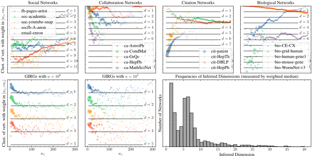
Figure 1: First row: our test statistic for different choices of wc in real-world networks. The size of the circles indicates the number of vertices in the induced subgraph of vertices with weight in [wc, cwc] for c = 1.15. Dashed lines show a lower bound on the expected value of our test statistic for a GIRG generated in dimension d, i.e (3/4)d . Second row, left: the same procedure for synthetic networks, generated with the algorithm of [Bl¨asius et al., 2022] using β = 2.5, α = 10 and average degree 10. Second row, right: distribution of the inferred dimension of 2976 real-world networks from the dataset of [Bl¨asius and Fischbeck, 2022].

6 FutureWork

A large body of work has been devoted to understanding for which asymptotic behavior of d geometry is detectable in spherical random geometric graphs (SRGGs) for homogeneous weights. While the parameter regime where these graphs lose geometry in the dense case, i.e. the case where the edge probability is constant and does not depend on n, is well understood [Devroye et al., 2011; Bubeck et al., 2016; Liu and R´acz, 2023b], it is unclear what happens in the sparse case (where the marginal connection probability is proportional to 1/n) and progress has been made only recently [Brennan et al., 2020; Liu et al., 2022].

On the other hand, research devoted to studying the influence of the dimension on random geometric graphs in the case of inhomogeneous weights is sparse. We gave first results in this regard by studying how the clustering coefficient depends on d and showed that the dimension can be detected by means of statistical testing assuming that d = o(log(n)), which is a valid assumption for realistic data. It is interesting to study under which conditions the geometry remains detectable if d = Ω(log(n)) and under which circumstances the model converges to its non-geometric counterpart with respect to the total variation distance of the distributions over the produced graphs as previously studied for spherical random graphs. Also, to determine what differences arise when using the torus instead of the sphere as the underlying metric space and which influence different norms have in this regard.

Noisy settings have also been considered in the context of testing for geometry in random graphs [Liu and R´acz, 2023a]. The GIRG model comes with a natural way of modelling noise in the form of an (inverse) temperature parameter α > 1 [Keusch, 2018]. As higher temperatures diminish clustering in addition to the effects induced by the dimension, it would be relevant to generalize our results to the case of non-zero temperatures and to investigate how the effects of high temperature can be distinguished from that of high dimension.

Finally, our experiments indicate that some real-world networks behave differently than GIRGs when being subjected to our test. One possible explanation is the non-zero assortativity of many real networks. Therefore, we would like to understand how this parameter influences our test and how the GIRG model can be extended by further parameters that allow adjusting assortativity and related properties.

Ethical Statement

There are no ethical issues.

Aknowledgements

Tobias Friedrich was funded by project No. 390859508 of the German Research Foundation. Andreas G¨obel was funded by the project PAGES (project No. 467516565) of the German Research Foundation (DFG). We thank Marcos Kiwi for fruitful discussions related to this work.