
SVD-AE: Simple Autoencoders for Collaborative Filtering
Proceedings of the Thirty-Third International Joint Conference on Artificial Intelligence. Main Track. Pages 2054-2062.
https://doi.org/10.24963/ijcai.2024/227
Keywords
- Multidisciplinary Topics and Applications: MTA: Web and social networks
- Data Mining: DM: Information retrieval
- Data Mining: DM: Collaborative filtering
Abstract
Collaborative filtering (CF) methods for recommendation systems have been extensively researched, ranging from matrix factorization and autoencoder-based to graph filtering-based methods. Recently, lightweight methods that require almost no training have been recently proposed to reduce overall computation. However, existing methods still have room to improve the trade-offs among accuracy, efficiency, and robustness. In particular, there are no well-designed closed-form studies for balanced CF in terms of the aforementioned trade-offs. In this paper, we design SVD-AE, a simple yet effective singular vector decomposition (SVD)-based linear autoencoder, whose closed-form solution can be defined based on SVD for CF. SVD-AE does not require iterative training processes as its closed-form solution can be calculated at once. Furthermore, given the noisy nature of the rating matrix, we explore the robustness against such noisy interactions of existing CF methods and our SVD-AE. As a result, we demonstrate that our simple design choice based on truncated SVD can be used to strengthen the noise robustness of the recommendation while improving efficiency. Code is available at https://github.com/seoyoungh/svd-ae.
- [Amatriain et al., 2009a] Xavier Amatriain, Josep M Pujol, and Nuria Oliver. I like it... i like it not: Evaluating user ratings noise in recommender systems. In International Conference on User Modeling, Adaptation, and Personal- ization, 2009.
- [Amatriain et al., 2009b] Xavier Amatriain, Josep M Pujol, Nava Tintarev, and Nuria Oliver. Rate it again: increasing recommendation accuracy by user re-rating. In RecSys, 2009.
- [Cho et al., 2011] Eunjoon Cho, Seth A Myers, and Jure Leskovec. Friendship and mobility: user movement in location-based social networks. In KDD, 2011.
- [Choi and Ryu, 2023] Jeongwhan Choi and Duksan Ryu. Qos-aware graph contrastive learning for web service rec- ommendation. In 2023 30th Asia-Pacific Software En- gineering Conference (APSEC), pages 171-180. IEEE, 2023.
- [Choi et al., 2021] Jeongwhan Choi, Jinsung Jeon, and Noseong Park. LT-OCF: Learnable-time ode-based col- laborative filtering. In CIKM, 2021.
- [Choi et al., 2023a] Jeongwhan Choi, Seoyoung Hong, Noseong Park, and Sung-Bae Cho. Blurring-sharpening process models for collaborative filtering. In SIGIR, 2023.
- [Choi et al., 2023b] Jeongwhan Choi, Hyowon Wi, Chae- jeong Lee, Sung-Bae Cho, Dongha Lee, and Noseong Park. Rdgcl: Reaction-diffusion graph contrastive learning for recommendation. arXiv preprint arXiv:2312.16563, 2023.
- [Feng et al., 2018] Xu Feng, Wenjian Yu, and Yaohang Li. Faster matrix completion using randomized svd. In 2018 IEEE 30th International conference on tools with artificial intelligence (ICTAI), pages 608-615. IEEE, 2018.
- [Halko et al., 2011] Nathan Halko, Per-Gunnar Martinsson, and Joel A Tropp. Finding structure with randomness: Probabilistic algorithms for constructing approximate ma- trix decompositions. SIAM review, 53(2):217-288, 2011.
- [Harper and Konstan, 2015] F Maxwell Harper and Joseph A Konstan. The movielens datasets: History and context. Acm Transactions on Interactive Intelligent Systems, 2015.
- [He et al., 2017] Xiangnan He, Lizi Liao, Hanwang Zhang, Liqiang Nie, Xia Hu, and Tat-Seng Chua. Neural collabo- rative filtering. In TheWebConf, 2017. [He et al., 2020] Xiangnan He, Kuan Deng, Xiang Wang, Yan Li, Yongdong Zhang, and Meng Wang. LightGCN: Simplifying and powering graph convolution network for recommendation. In SIGIR, 2020.
- [Hong et al., 2022] Seoyoung Hong, Minju Jo, Seungji Kook, Jaeeun Jung, Hyowon Wi, Noseong Park, and Sung- Bae Cho. Timekit: A time-series forecasting-based up- grade kit for collaborative filtering. In IEEE International Conference on Big Data (Big Data), 2022.
- [Hong et al., 2024] Seoyoung Hong, Jeongwhan Choi, Yeon-Chang Lee, Srijan Kumar, and Noseong Park. SVD-AE: Simple autoencoders for collaborative filtering. arXiv preprint arXiv:2405.04746, 2024.
- [Jain et al., 2016] Himanshu Jain, Yashoteja Prabhu, and Manik Varma. Extreme multi-label loss functions for rec- ommendation, tagging, ranking & other missing label ap- plications. In KDD, 2016.
- [Kim et al., 2023] Min-Jeong Kim, Yeon-Chang Lee, and Sang-Wook Kim. Trustsgcn: Learning trustworthiness on edge signs for effective signed graph convolutional net- works. In SIGIR, 2023.
- [Kipf and Welling, 2017] Thomas N. Kipf and Max Welling. Semi-supervised classification with graph convolutional networks. In ICLR, 2017.
- [Kong et al., 2022] Taeyong Kong, Taeri Kim, Jinsung Jeon, Jeongwhan Choi, Yeon-Chang Lee, Noseong Park, and Sang-Wook Kim. Linear, or non-linear, that is the ques- tion! In WSDM, pages 517-525, 2022.
- [Lee et al., 2021] Dongha Lee, SeongKu Kang, Hyunjun Ju, Chanyoung Park, and Hwanjo Yu. Bootstrapping user and item representations for one-class collaborative filtering. In SIGIR, 2021.
- [Lee et al., 2024] Chaejeong Lee, Jeongwhan Choi, Hyowon Wi, Sung-Bae Cho, and Noseong Park. Stochastic sam- pling for contrastive views and hard negative samples in graph-based collaborative filtering. arXiv preprint arXiv:2405.00287, 2024.
- [Liang et al., 2018] Dawen Liang, Rahul G Krishnan, Matthew D Hoffman, and Tony Jebara. Variational autoen- coders for collaborative filtering. In TheWebConf, 2018.
- [Mao et al., 2021] Kelong Mao, Jieming Zhu, Xi Xiao, Biao Lu, Zhaowei Wang, and Xiuqiang He. UltraGCN: ultra simplification of graph convolutional networks for recom- mendation. In CIKM, 2021.
- [Moon et al., 2023] Jaewan Moon, Hye-young Kim, and Jongwuk Lee. It's enough: Relaxing diagonal constraints in linear autoencoders for recommendation. In SIGIR, 2023.
- [Murakami and Aibara, 1987] Kenji Murakami and Tsune- hiro Aibara. An improvement on the moore-penrose gen- eralized inverse associative memory. IEEE transactions on systems, man, and cybernetics, 17(4):699-707, 1987.
- [Ortega et al., 2018] Antonio Ortega, Pascal Frossard, Jelena Kovačević, José MF Moura, and Pierre Vandergheynst. Graph signal processing: Overview, challenges, and appli- cations. Proceedings of the IEEE, 106(5):808-828, 2018.
- [Park et al., 2024] Jin-Duk Park, Yong-Min Shin, and Won- Yong Shin. Turbo-cf: Matrix decomposition-free graph filtering for fast recommendation. arXiv preprint arXiv:2404.14243, 2024.
- [Peng et al., 2022] Shaowen Peng, Kazunari Sugiyama, and Tsunenori Mine. Svd-gcn: A simplified graph convolution paradigm for recommendation. In CIKM, 2022.
- [Rendle et al., 2012] Steffen Rendle, Christoph Freuden- thaler, Zeno Gantner, and Lars Schmidt-Thieme. BPR: Bayesian personalized ranking from implicit feedback. arXiv preprint arXiv:1205.2618, 2012.
- [Sachdeva et al., 2022] Noveen Sachdeva, Mehak Preet Dhaliwal, Carole-Jean Wu, and Julian McAuley. Infinite recommendation networks: A data-centric approach. In NeurIPS, 2022.
- [Said et al., 2012] Alan Said, Brijnesh J Jain, Sascha Narr, and Till Plumbaum. Users and noise: The magic barrier of recommender systems. In International Conference on User Modeling, Adaptation, and Personalization, 2012.
- [Sar Shalom et al., 2015] Oren Sar Shalom, Shlomo Berkovsky, Royi Ronen, Elad Ziklik, and Amir Amihood. Data quality matters in recommender systems. In RecSys, 2015.
- [Sharma et al., 2022] Kartik Sharma, Yeon-Chang Lee, Sivagami Nambi, Aditya Salian, Shlok Shah, Sang-Wook Kim, and Srijan Kumar. A survey of graph neural net- works for social recommender systems. arXiv preprint arXiv:2212.04481, 2022.
- [Shen et al., 2021] Yifei Shen, Yongji Wu, Yao Zhang, Cai- hua Shan, Jun Zhang, B Khaled Letaief, and Dongsheng Li. How powerful is graph convolution for recommenda- tion? In CIKM, 2021.
- [Shin et al., 2024] Yehjin Shin, Jeongwhan Choi, Hyowon Wi, and Noseong Park. An attentive inductive bias for sequential recommendation beyond the self-attention. In AAAI, 2024.
- [Shishkin et al., 2019] Serge L Shishkin, Arkadi Shalaginov, and Shaunak D Bopardikar. Fast approximate truncated svd. Numerical Linear Algebra with Applications, 2019.
- [Steck, 2019] Harald Steck. Embarrassingly shallow autoen- coders for sparse data. In TheWebConf, 2019.
- [Steck, 2020] Harald Steck. Autoencoders that don't overfit towards the identity. In NeurIPS, 2020.
- [Stiles and Denq, 1985] Gardiner S Stiles and Dong-Lih Denq. On the effect of noise on the moore-penrose gener- alized inverse associative memory. IEEE transactions on pattern analysis and machine intelligence, 1985.
- [Wang et al., 2019] Xiang Wang, Xiangnan He, Meng Wang, Fuli Feng, and Tat-Seng Chua. Neural graph col- laborative filtering. In SIGIR, 2019.
- [Ying et al., 2018] Rex Ying, Ruining He, Kaifeng Chen, Pong Eksombatchai, William L Hamilton, and Jure Leskovec. Graph convolutional neural networks for web- scale recommender systems. In KDD, 2018.
References were extracted automatically from the PDF and may contain errors.
Full text extracted automatically from the PDF; figures, tables and equations may differ. The PDF is the version of record.
1 Introduction
Recommender systems have been utilized extensively in a variety of service platforms, including e-commerce and social media [Ying et al., 2018; Sharma et al., 2022; Choi and Ryu, 2023; Shin et al., 2024]. Collaborative Filtering (CF), a crucial task for recommendation, typically learns latent vectors (i.e., embeddings) of users and items from their prior user-item interactions and provides personalized preferred recommendations [Rendle et al., 2012; He et al., 2017]. Since the user-item interaction matrix can be represented as a binary graph, graph-based CF, which learns user and item embeddings using graph convolutional neural networks
∗Work done while at Yonsei University.
†Corresponding author.
| GF-CF | EASE | ∞-AE | SVD-AE | |
|---|---|---|---|---|
| Closed-form Solution Autoencoder-based Using SVD Using Neural Networks Inference Target | ✓ ✗ ✓ ✗ Item-item | ✓ ✓ ✗ ✗ Item-item | ✓ ✓ ✗ ✓ User-user | ✓ ✓ ✓ ✗ User-item |
(GCNs) [Kipf and Welling, 2017], has been widely studied recently [He et al., 2020; Lee et al., 2021; Choi et al., 2021; Kong et al., 2022; Hong et al., 2022; Choi et al., 2023b; Kim et al., 2023; Lee et al., 2024].
At the same time, the escalating expense of training models on massive datasets, including billions of user-item interactions, has become a difficulty in the study of recommender systems. Since LightGCN [He et al., 2020] simplified the GCN-based CF and improved its performance by eliminating nonlinear activation functions and feature transformations, recent works have attempted to make LightGCN more lightweight [Mao et al., 2021; Peng et al., 2022]. Despite these advancements, learning-based approaches still have drawbacks in that they need a lot of time and computation since they require training.
Therefore, various research has provided lightweight and effective computing approaches based on closed-form solutions to lessen the computational complexity [Steck, 2019; Shen et al., 2021; Sachdeva et al., 2022; Choi et al., 2023a]. GF-CF [Shen et al., 2021] designs a simple and computationally efficient framework that uses various graph filters. On the other hand, autoencoders (AE) are also used to construct the closed-form solution for CF. EASE [Steck, 2019] discovers the closed-form solution of the shallow AE-based recommender system by solving its linear regression-based formulation via Lagrangian multipliers. ∞-AE [Sachdeva et al., 2022] suggests adopting the neural tangent kernel (NTK) to obtain the closed-form solution of the autoencoder with an infinitely-wide bottleneck layer for recommendation.
While these methods exhibit successful considerations for efficiency and performance in their design, they face challenges in achieving excellent generalization abilities due to the prevalent presence of noisy interactions in the recommendation data. It is well-known that a user-item interaction matrix, R ∈ {0, 1}|U|×|I| , where U is a set of users and I is a set of items, often contains noise [Said et al., 2012]. That is, an interaction does not necessarily mean that a user is satisfied with an item [Amatriain et al., 2009b; Sar Shalom et al., 2015]. In this case, EASE and ∞-AE employ straightforward reconstruction of R, which can lead to noisy interactions if not properly controlled [Steck, 2020].
In this work, we aim to explore the way for the best overall balance between accuracy, computational speed, and noise robustness. Toward this goal, we propose an SVD-AE for CF, whose optimal solution can be analytically defined with the truncated SVD, to effectively exclude the noise in the original rating matrix when inferring ˆR. Additionally, our SVDAE directly reveals ˆR fromRwithout any intermediate steps, thus reducing the computation time, whereas other methods, e.g., GF-CF, EASE, and ∞-AE, require obtaining the itemitem or user-user similarity matrix from R. We experimentally show that our simple design choice based on truncated SVD leads to a practical way to i) enhance the balance among recommendation accuracy, computation time, and robustness, and ii) enable obtaining a closed-form solution devoid of any parameters to train. In Table 1, we compare our SVD-AE with existing lightweight methods, which will be discussed in more detail in Sections 3.1 and 3.2.
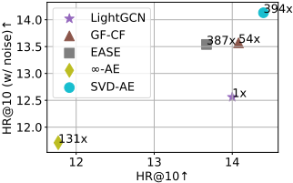
The experiments with 8 baselines on 4 datasets demonstrate that our SVD-AE marks the best place for HR@10, NDCG@10, and PSP@10 by non-trivial margins. Furthermore, we study the robustness against the addition of random noisy interactions of all the baselines and our SVD-AE. As shown in Figure 1, SVD-AE has the fastest computation time (spec., 394 times quicker than LightGCN), provides the best recommendation accuracy (HR@10), and performs best even with the addition of random noisy interactions, demonstrating its robustness.
Our contributions can be summarized as follows:
- Novel Closed-form Solution for CF: Our SVD-AE, a simple but efficient linear AE using SVD, has a closedform solution for CF. We also devise a generalized AE form that subsumes all existing AE-based CF methods.
- Robust Methodology: We discuss how to use the truncated SVD to avoid potential overfitting by the noisy interactions. Through in-depth analyses, we also investigate the superior robustness of AE-based recommendation methods to noise, including our SVD-AE.
- Comprehensive Validation: Our method outperforms all baselines in all benchmark datasets for HR@10, NDCG@10, and PSP@10. Furthermore, compared to many other existing methods, the computation time is much shorter as it has an even simpler closed-form solution than others. Therefore, our method offers the best overall balance between the accuracy of the recommendation, the computation time, and the noise robustness.
2 RelatedWork &Preliminaries
2.1 Lightweight Collaborative Filtering
In recent years, several CF methods have been developed to build lightweight recommender systems [Shen et al., 2021; Choi et al., 2023a; Park et al., 2024]. First, GF-CF [Shen et al., 2021] designed a simple and computationally efficient framework that leverages various graph filters. Other methods typically employ autoencoder approaches based on linear regression [Steck, 2019; Sachdeva et al., 2022]. EASE [Steck, 2019] suggested a shallow autoencoder that simply calculates an item-item similarity matrix using ordinary least squares regression with a closed-form solution. They also used Lagrangian multipliers to constrain the selfsimilarity of each item in the input and output layer to zero. Recently, ∞-AE [Sachdeva et al., 2022] adopted the NTK to obtain the closed-form solution of the autoencoder with an infinitely-wide bottleneck layer for recommendation. RLAE and RDLAE [Moon et al., 2023] extended EASE by adjusting the degree of diagonal constraints through tuning for L2 regularization with random dropout.
2.2 Generalized Linear Autoencoder for Recommender Systems
In this section, we describe a generalized linear autoencoder for recommender systems and demonstrate how simple regression methods solve the problem of finding the optimal model. We then present existing methods to solving the linear regression.
The objective function of linear autoencoder is written as:
where C denotes a set of constraints. R ∈ {0, 1}|U|×|I| and ˆR ∈ {0, 1}|U|×|I| represent a given user-item interaction matrix and a reconstructed interaction matrix, respectively. U and I denote sets of users and items, respectively.
Many existing recommendation methods can be generalized into the above form with specific choices for their own constraints. Their closed-form solutions for optimal ˆR are given by:
where the specific interpretations are:
- In the case of EASE [Steck, 2019], ˆP = (RT R+λI)-1 , λ is a hyperparameter for regularization, and ⊘ denotes the element-wise division.
- In the case of ∞-AE [Sachdeva et al., 2022], K ∈ R|U|×|U| is a Gram matrix that represents the similarity of users, i.e., Ku,v := K(Ru,Rv) for all u, v ∈ U. K denotes a NTK, K : R|I| × R|I| ↦→ R over an Reproducing Kernel Hilbert Space H of a single-layer autoencoder with an activation function σ. A closed-form solution is given by K(Ru, Rv) = ˜σ(RTu Rv)+˜σ′ (RTu Rv) · RTu Rv. ˜σ represents the dual activation of σ and ˜σ′ represents its derivative. λ is a regularization parameter.
- In the case of our SVD-AE, which will be described in detail in Section 3, ˜R is a normalized rating matrix given by ˜R=D- 12 U RD- 12 I . DU = diagMat(R·1) andDI = diagMat(1T R) are degree matrices. Q ∈ R|U|×m and V ∈ R|I|×m are the top-m singular vectors, and ˜Σ denotes the top-m singular values of ˜R.
For all methods, linear regression is used to discover the closed-form solution of learning the optimal ˆR. We show how two simple regression methods - ridge regression and kernelized ridge regression - solve the problem in the closed-form in the following.
Ridge Regression. EASE applies ordinary least squares regression and derives B using the following convex objective:
where ∥ · ∥F denotes the Frobenius norm and λ is the regularization parameter. The problem in Eq. (3) is a simple ridge regression and the solution is well-known as follows:
EASE also includes Lagrangian multipliers into the problem to fulfill the zero diagonal constraints in Eq. (4). This is important in order to avoid trivial solution B = I.
Kerenelized Ridge Regression. By using the estimated NTK, ∞-AE conducts Kernelized Ridge Regression (KRR) which is the same as training an infinitely-wide autoencoder for an infinite number of SGD steps. They reduce the problem to KRR as follows:
where α := [α1; α2...; α|U|] ∈ R|U|×|I| are the set of dual parameters to estimate and λ is a regularization constant. The KRR problem in Eq. (6) has a closed-form solution given by ˆα = (K+ λI)-1 · R s.t. Ku,v := K(Ru, Rv) ∀u, v.
3 SVD-AE
In this section, we describe our three design goals, followed by our detailed method design and its low-rank approximation. Finally, we discuss the advantages of SVD-AE and explore how it relates to other recommendation methods.
DesignGoals. Our proposed problem formulation has been designed for the following three design goals:
- (Robustness) Its problem formulation should include an effective inductive bias that can lead to high noise robustness;
- (Complexity) Its closed-form solution should be no more complicated than existing methods based on different closed-form solutions, e.g., EASE and ∞-AE;
- (Accuracy) Its recommendation accuracy ought to be comparable to that of existing CF methods.
Method Design. Our SVD-AE solves yet another linear regression problem for the recommendation - however, its problem formulation can still be in the generalized linear regression regime of Eq. (1), i.e.,
where ˜R is a normalized adjacency matrix given by ˜R = D- 12 U RD- 1 2 I . DU = diagMat(R · 1) and DI = diagMat(1T R) are degree matrices.
Based on Theorem 1 and 2, we can derive the closed-form solution of B as follows:
Theorem 1. The least squares solutions of the minimum norm of the linear system ˜RB = R is given by
where ˜R+ is the the pseudo-inverse of ˜R.
Theorem2. Let ˜Rbe a normalized adjacency matrix and the SVD of ˜R be
where Q, V are both orthogonal matrices and Σ = diagMat(σ1, ..., σM) is a diagonal matrix containing the singular values of ˜R. Then the pseudo-inverse of ˜R denoted by ˜R+ is defined as:
where Σ+ is given by Σ+ = diagMat(1/σ1, ..., 1/σM).
Low-rank Inductive Bias. However, it is known that the pseudo-inverse can provide serious effects when used in the presence of noise [Stiles and Denq, 1985; Murakami and Aibara, 1987]. The truncated SVD is one method for stabilizing the pseudo-inverse among others.
The truncated SVD uses only the first m columns of Q and V and the first m largest singular values. The relatively large and small singular values of the matrix with rank M typically cluster into two groups, i.e.,
Noise reduction can be executed by utilizing only the significant components represented by m singular values from the larger group, considering the smaller group as noise. Truncated SVD is widely used in recommender systems to handle noise in the rating matrix R [Shen et al., 2021; Peng et al., 2022]. Since the rating matrix is typically vast and sparse, it is also useful for speeding up calculations and information retrieval.
We use the normalized adjacency matrix whose singular values are between 0 and 1 as shown in the next theorem. This avoids having singular values that are too small or large.
Theorem 3. Let σ1 ≥ σ2 ≥ ... ≥ σM be the singular values of ˜R given by ˜R=D- 1 2 U RD- 12 I , then
Using the truncated SVD, Q ∈ R|U|×m and V ∈ R|I|×m are the top-m singular vectors and ˜Σ denotes the top-m singular values of ˜R given by ˜Σ = diagMat(σ1, ..., σm). Thus, the following is the reconstructed (or inferred) interaction matrix ˆR for recommendation:
Proofs of the theorems are in our full paper [Hong et al., 2024, Appendix B].
3.1 Why SVD-AE Achieves the Best Balance?
The Presence of Noise. Many algorithms used in recommender systems utilize observed ratings to predict unknown ratings. The user ratings can be seen as the ground truth of the user's preference, which is an underlying assumption in this method. However, given the presence of noisy data, inferring unknown ratings is challenging. A user-item interaction record does not always mean that users are satisfied with consumed items, which frequently happens for implicit interactions. Users are also inconsistent in giving their feedback, creating an undetermined amount of noise that makes it more challenging to infer unreported ratings [Amatriain et al., 2009b; Sar Shalom et al., 2015; Said et al., 2012; Amatriain et al., 2009a]. Therefore, the two types of interaction noises can be summarized as follows:
- (Noisy 1 in R) A user is not satisfied with an item, but an interaction is observed between them;
- (Noisy 0 in R) A user will be satisfied with an item, but there are no observed interactions between them. The ultimate goal of recommendation is to accurately reveal these hidden interactions.
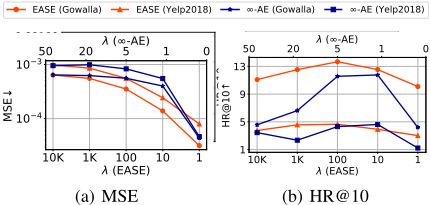
Here, one can argue that EASE and ∞-AE address these noises by preventing overfitting through the regularization parameter λ. In Figure 2, we show that minimizing the Mean Squared Error (MSE) loss in Eq. (1) does not guarantee the recommendation performance. We can observe that performance does not increase when EASE and ∞-AE use smaller λ to get closer to R, a trivial solution of ˆR. For all cases, the performance is at the lowest even when the smallest λ is applied. Using the appropriate λ leads to higher performance by avoiding overfitting the noise-inherent original rating matrix.
However, rather than using a regularization parameter, we adopt the truncated SVD to strongly and directly prevent overfitting of noisy interactions. In the perspective of signal processing [Ortega et al., 2018], the above two types of noises correspond to high-frequency signals in R. In other words, they typically make local abrupt changes in the adjacency structure of R. For instance, the second type means that a hidden element (edge) of R is zero when its incident elements (edges) frequently have 1 - the first type can also be interpreted similarly. One effective noise removal method is to smooth out those local large changes (i.e., high-frequency signals) by utilizing only the m lowest frequency signals. To this end, our design is based on the effective low-rank inductive bias based on the truncated SVD with a rank parameter of m. Among various possible inductive biases, we have chosen the (low-rank) truncated SVD for its effectiveness.
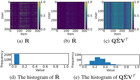
Figures 3 (a), (b), and (c) show the smoothing effect of the truncated SVD. We discover that stable structured data extraction is possible by reconstructing the adjacency matrix using the truncated SVD. The truncated SVD converts the original data into the good representation by reducing noise. Comparing Figures 3 (d) and (e), it is clear that the reconstructed representation (i.e., Figure 3 (e)) has a range of values as opposed to the existing data distribution (i.e., Figure 3 (d)), which had only values very close to zero.
Computational Cost. In this part, we examine the computational cost of SVD-AE. We use a fast randomized truncated SVD [Halko et al., 2011] and its computational complexity is O(|U| · |I| · log(m) + (|U| + |I|) · m2 ). This can be done in the pre-processing step - there exist even more lightweight methods to approximate the truncated SVD [Shishkin et al., 2019; Feng et al., 2018], and one can try to further decrease the time complexity by using them. In the case of EASE and ∞-AE, they need to compute the matrix inversion of the data Gram matrix, RT R ∈ R|I|×|I| or RRT ∈ R|U|×|U| . Then the computation complexity would be O(|I|2.376 ) or O(|U|2.376 ) that are computationally-expensive. However, since we do not have to compute the matrix inversion, the computational cost is significantly reduced. The overall computation cost comes out to be O(|U| · |I|2 ). The computation complexity of EASE is O(|I| · (|I| - 1)2.376 ) with the additional cost O(|U| · |I|2 ) for pre-processing step whereas ∞-AE's cost is O(|U|2 · |I| + |U|2.376 ).
3.2 Relation to Other Methods
Table 1 summarizes the key distinctions between our SVDAE and current lightweight methods. We will now explore their relationships and compare SVD-AE to others.
EASE, ∞-AE, and SVD-AE share the CF paradigm, utilizing a shallow autoencoder-based linear regression for problem resolution, leading to closed-form optimization. EASE and ∞-AE are based on ridge regression with the regularization parameter λ to avoid overfitting. Unlike previous methods, SVD-AE does not require an additional regularizer by directly using the truncated SVD as a low-rank inductive bias, to avoid overfitting more sophisticated. As discussed earlier in The Presence of Noise, this design choice is based on the smoothing effect and the efficient low-rank inductive bias of truncated SVD. For ∞-AE, it needs to build a neural network to use NTK, but other methods can reconstruct the matrix using a simple matrix computation. This complexity results in ∞-AE having longer execution times with large datasets than EASE or SVD-AE (see Section 4.3).
GF-CF [Shen et al., 2021] is a graph filter-based model, which is a combination of the linear graph filter and the ideal low-pass graph filter. In GF-CF, the truncated SVD is used to construct an ideal low-pass graph filter rather than to prevent overfitting. In other words, it is used as an auxiliary to add information to the linear graph filter, rather than as the main mechanism. However, in SVD-AE, the information obtained solely through the truncated SVD is directly used as the main objective. This design choice not only simplifies the process but also enhances efficiency, as it employs an autoencoder and involves only a linear regression problem. It is in contrast to the graph-based approach, such as GF-CF, which typically requires more complex designs and computational steps.
Additionally, comparing low-rank and full-rank methods is another intriguing aspect of our research. SVD-AE is designed on top of our low-rank inductive bias, while GFCF also partially utilizes it. This contrasts EASE and ∞- AE, which use full-rank information. Moreover, ∞-AE is an over-parameterized model with an infinitely wide layer. Our experiments will show that low-rank methods, due to their low-rank inductive bias, outperform full-rank and overparametrized methods for sparse data.
Finally, using a Gram matrix is another distinctive feature of these approaches. In recommender systems, it is common to compute an item-item or user-user similarity matrix from which to derive a new user-item interaction matrix. EASE and GF-CF utilize an item-item matrix, while ∞-AE uses a user-user matrix. SVD-AE does not use any of them but directly infers user-item interactions, which reduces the overall computation cost as shown in Section 3.1.
4 Experiments
In this section, we describe the experimental settings and then compare our SVD-AE with state-of-the-art CF methods. We also discuss our study of the robustness of various algorithms.
4.1 Experimental Environments
Datasets. In our experiments, we use four of the most widely used publicly available datasets [Cho et al., 2011; Harper and Konstan, 2015]: Gowalla, Yelp2018, ML-1M, and ML-10M. More details on datasets are in our full paper [Hong et al., 2024, Appendix C.2].
Evalutation Protocol. We compare SVD-AE with 8 baselines: MF-BPR [Rendle et al., 2012], NeuMF [He et al., 2017], NGCF [Wang et al., 2019], LightGCN [He et al., 2020], GF-CF, MultVAE [Liang et al., 2018], EASE, and ∞- AE. We provide details on baselines and their hyperparameter configurations in our full paper [Hong et al., 2024, Appendix C.3]. For a fair comparison with previous studies, we use the same train/validation/test splits as done in [He et al., 2020; Shen et al., 2021; Sachdeva et al., 2022]. We evaluate the accuracy of all of the methods using HR@k, NDCG@k, and PSP@k [Jain et al., 2016].
Implementation Details. We need to take m as a rank parameter when running the truncated SVD. For simplicity, we use m = ⌊γ × min(|U|, |I|)⌉, where ⌊...⌉ function denotes the rounding function. We search for γ in the range of [0.01, 0.02, 0.03, 0.04, 0.05] with the validation set with HR@10. Note that γ is our sole hyperparameter, and γ = 0.04 is universally optimal for all datasets, simplifying the selection of suitable rank parameter m.
4.2 Performance Comparison
The performance of the proposed method and other benchmark models are shown in Table 2. Overall, our SVDAE achieves comparable to or better performance than other various methods. SVD-AE yields the best performance for HR@10, NDCG@10, and PSP@10 across all datasets. Among all baselines, GF-CF performs well on the relatively sparse datasets, Gowalla and Yelp2018. AE-based models such as EASE and ∞-AE perform rather poorly for these datasets. SVD-AE performs well on sparse datasets compared to other AE-based models, and outperforms EASE and ∞-AE on Gowalla by 5.3% and 22.3%, respectively, in terms of HR@10. In less sparse datasets like ML-1M and ML10M, where user-item interactions are comparatively sufficient, AE models outperform non-AE models. ∞-AE and EASE show good performance on ML-1M and ML-10M. But once again, SVD-AE has the greatest performance aside from HR@100 on ML-1M. In highly sparse datasets, AE-based models struggle to reconstruct the rating matrix for deriving the inferred matrix. However, SVD-AE maintains consistent performance across dataset types, possibly owing to our lowrank inductive bias.
| Dataset | Measure | MF-BPR | NeuMF | NGCF | LightGCN | GF-CF | MultVAE | EASE | ∞-AE | SVD-AE |
|---|---|---|---|---|---|---|---|---|---|---|
| Gowalla | HR@10 | 12.08 | 8.87 | 11.70 | 14.00 | 14.08 | 11.88 | 13.67 | 11.77 | 14.40 |
| HR@100 | 32.84 | 27.25 | 32.22 | 37.40 | 38.84 | 33.56 | 35.74 | 34.20 | 37.34 | |
| NDCG@10 | 12.09 | 8.27 | 11.70 | 13.77 | 13.50 | 11.30 | 13.15 | 10.84 | 13.94 | |
| NDCG@100 | 18.44 | 13.96 | 17.95 | 21.04 | 21.25 | 18.11 | 20.08 | 17.97 | 21.15 | |
| PSP@10 | 1.92 | 1.37 | 1.76 | 2.26 | 2.47 | 2.09 | 2.31 | 2.02 | 2.48 | |
| Yelp2018 | HR@10 | 3.86 | 3.25 | 3.68 | 4.32 | 4.87 | 4.31 | 4.65 | 4.62 | 4.90 |
| HR@100 | 16.97 | 14.39 | 16.88 | 19.01 | 20.86 | 18.75 | 17.74 | 18.33 | 19.79 | |
| NDCG@10 | 3.70 | 3.08 | 3.50 | 4.19 | 4.66 | 4.10 | 4.55 | 4.48 | 4.74 | |
| NDCG@100 | 8.50 | 7.16 | 8.33 | 9.57 | 10.53 | 9.37 | 9.37 | 9.54 | 10.22 | |
| PSP@10 | 0.34 | 0.27 | 0.32 | 0.39 | 0.44 | 0.43 | 0.42 | 0.43 | 0.45 | |
| ML-1M | HR@10 | 28.49 | 27.95 | 28.40 | 29.07 | 30.81 | 27.86 | 30.43 | 31.15 | 31.79 |
| HR@100 | 57.21 | 54.24 | 57.58 | 57.62 | 59.10 | 57.67 | 57.74 | 60.75 | 59.33 | |
| NDCG@10 | 29.84 | 29.36 | 29.43 | 30.30 | 32.37 | 28.44 | 31.90 | 32.27 | 33.55 | |
| NDCG@100 | 39.47 | 37.98 | 39.27 | 39.95 | 42.00 | 39.34 | 40.95 | 42.54 | 42.57 | |
| PSP@10 | 2.89 | 2.75 | 2.90 | 3.01 | 3.17 | 3.13 | 3.16 | 3.22 | 3.22 | |
| ML-10M | HR@10 | 33.28 | 25.75 | 34.79 | 35.10 | 34.20 | 36.30 | 35.83 | 36.76 | |
| HR@100 | 64.16 | 58.63 | 64.11 | 64.23 | 64.55 | 64.78 | 64.48 | 64.80 | ||
| NDCG@10 | 33.58 | 25.32 | Timed Out | 35.60 | 36.02 | 34.48 | 37.63 | 36.93 | 37.75 | |
| NDCG@100 | 44.32 | 36.90 | 46.14 | 45.71 | 45.23 | 46.74 | 46.27 | 46.97 | ||
| PSP@10 | 4.60 | 3.52 | 4.69 | 4.73 | 4.82 | 4.76 | 4.74 | 4.93 |
| Model | ML-1M | ML-10M | ||
|---|---|---|---|---|
| Pre-processing | Training | Pre-processing | Training | |
| MF-BPR | N/A | 24.48m | N/A | 48.56h |
| NeuMF | N/A | 2.68h | N/A | 145.98h |
| NGCF | N/A | 4.83h | N/A | Timed Out |
| LightGCN | N/A | 2.44h | N/A | 132.97h |
| GF-CF | 4.62s | 6.37s | 28.98s | 1260.80s |
| MultVAE | N/A | 221.78s | N/A | 1293.76s |
| EASE | 4.52s | 5.72s | 52.63s | 6.05s |
| ∞-AE | N/A | 2.24s | N/A | 388.39s |
| SVD-AE | 0.54s | 2.06s | 47.59s | 3.06s |
One can argue that the accuracy improvements of SVD-AE over baselines are often incremental. However, we emphasize that the goal of this work is to design a method that achieves a reasonable level of accuracy compared to baselines, while considerably diminishing computational time and improving robustness to noisy interactions, which will be validated in the subsequent sections.
4.3 Efficiency Comparison
We contrast the training time for our method with that of baseline models. For all models, we employ the same experimental setups and batch sizes. For runtime studies, we use the smallest and largest datasets, ML-1M and ML-10M.
Table 3 illustrates the huge discrepancy between the two methods-training models (i.e., MF-BPR, NeuMF, NGCF, LightGCN, and MultVAE) and non-training models (i.e., EASE, GF-CF, ∞-AE, and SVD-AE). The limitation of training models is clearly seen when the data size is huge. Notably, their efficiency may be acceptable for small datasets, but may take several days to train for large datasets. Especially in the case of NGCF, it is impracticable to train the model for ML-10M. Among the training models, MultVAE, the AE-based model shows a tolerable calculation time regardless of the size of the dataset.
The non-training models like GF-CF, EASE, and ∞-AE have relatively faster computation times. The presence of closed-form solutions makes this feasible. In the case of ∞- AE, however, compared to other AE-based models, it takes a lot longer to compute as the size of the data increased. This is because ∞-AE employs the NTK, making it more complex than lighter methods. Most importantly, our SVD-AE can achieve good performance in less time, which further illustrates the high efficiency of SVD-AE.
We also report pre-processing time as some methods including our method require pre-processing. GF-CF and SVDAE require the truncated SVD before training. In the case of EASE, it computes RT R in the pre-processing step. Table 3 shows that the time taken for the truncated SVD increases with the data size. However, since 10M interactions take only a minute, the procedure is not onerous.
4.4 Robustness Analyses
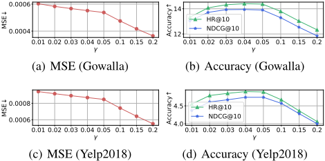
Robustness on Observed Noise. Similar to Figure 4, here we investigate the influence of the rank parameter γ of our SVD-AE. On all datasets, we examine the effectiveness of SVD-AE with different γ. More results in other datasets are in our full paper [Hong et al., 2024, Appendix D]. We observe that the MSE loss decreases as γ (consequently, m) increases. This is because the truncated SVD is performed as closely as possible to the original matrix as m increases. We can see, nevertheless, that recommendation performance is not always enhanced by using larger m. As the MSE loss decreases, the recommendation performance increases up to a certain level. However, beyond a certain threshold, we can observe a decline in the recommendation performance instead. This is because the noise from the rating matrix would be included in the reconstructed matrix if m is too large. Such an occurrence further demonstrates that minimizing MSE loss does not ensure that recommendations may work better, which is consistent with what we discovered in the previous experiments on existing AE-based recommender systems which is illustrated in Figure 2. Furthermore, it supports our low-rank inductive bias.
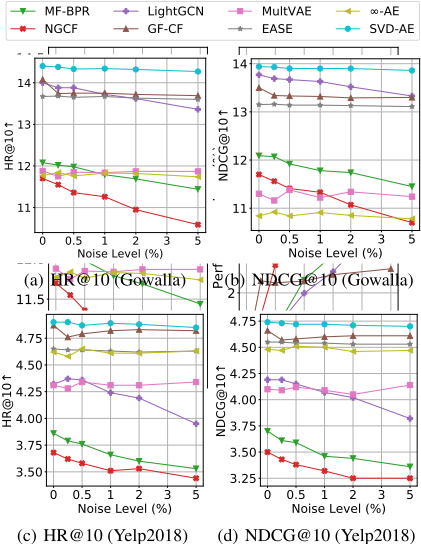
Robustness on Unobserved Noise. In this part, we study the noise robustness of various CF methods. To evaluate the robustness of the proposed method and baselines, we show the performance of all methods on Gowalla and Yelp2018 with different noise levels in Figure 5. To simulate the noise, we generate random user-item interactions from 0.5% to 5% of the dataset size, thereby adjusting the amount of noise to different dataset sizes.
We explore the robustness of four AE models, including MultVAE, EASE, ∞-AE, and our SVD-AE, and four non-AE models, including MF-BPR, NGCF, LightGCN, and GF-CF. Note that NeuMF is excluded for better visualization due to its significantly lower performance. In Figure 5, we can observe that our method can continue to perform steadily and competitively on noisy data of different degrees. We can see the greatest HR@10 and NDCG@10 are maintained regardless of the noise levels for Gowalla and Yelp2018.
On the other hand, a noteworthy feature is a significant disparity in noise robustness between AE and non-AE models. We discover that non-AE methods that disregard noise, such as MF-BPR, NGCF, and LightGCN, perform noticeably worse than the others when the noisy interactions are added. As a result, their HR@10 and NDCG@10 fall more significantly as the noise level increases. We can show that, among non-AE models, GF-CF is the most stable. We believe this is the indirect effect of using truncated SVD, although GF-CF
does not use it to avoid the overfitting problem.
Additionally, we can observe that AE-based models, including MultVAE, EASE, and ∞-AE, are consistently stable for various noise levels. However, as shown in Figure 5, they perform less reliably than SVD-AE. Notably, they also often perform worse than LightGCN and GF-CF in the experiment on Gowalla as shown in Figures 5 (a) and (b). Based on these observations, our SVD-AE provides the best recommendation accuracy while maintaining robust performance even with the addition of noise.
5 Conclusion
We proposed a simplified but efficient linear AE based on SVD and featuring a closed-form solution for CF. Our SVDAE outperforms various recommender systems including AEbased and non-AE models. Furthermore, compared to other methods, our method's runtime complexity is remarkably low. We discovered that our low-rank inductive bias via the truncated SVD makes it possible to obtain a closed-form solution and to effectively improve the robustness of the recommendation. Given the noisy nature of the rating matrix, we also discussed the overfitting issues with current recommender systems and presented the superior noise robustness of AE-based techniques, including SVD-AE. Our approach achieves the best balance between recommendation accuracy, computation time, and noise robustness. We expect much follow-up research work based on our observations of the new closed-form solution to the recommendation problem, in addition to the recent successes of developing lightweight methods with closed-form solutions.
Acknowledgements
This work was partly supported by Samsung Electronics Co., Ltd. (No. G01240136), the Korea Advanced Institute of Science and Technology (KAIST) grant funded by the Korea government (MSIT) (No. G04240001, Physics-inspired Deep Learning), and Institute for Information & Communications Technology Planning & Evaluation (IITP) grants funded by the Korea government (MSIT) (No. RS-2020-II201361, Artificial Intelligence Graduate School Program (Yonsei University)).
@inproceedings{ijcai2024p227,
  title     = {SVD-AE: Simple Autoencoders for Collaborative Filtering},
  author    = {Hong, Seoyoung and Choi, Jeongwhan and Lee, Yeon-Chang and Kumar, Srijan and Park, Noseong},
  booktitle = {Proceedings of the Thirty-Third International Joint Conference on
               Artificial Intelligence, {IJCAI-24}},
  publisher = {International Joint Conferences on Artificial Intelligence Organization},
  editor    = {Kate Larson},
  pages     = {2054--2062},
  year      = {2024},
  month     = {8},
  note      = {Main Track},
  doi       = {10.24963/ijcai.2024/227},
  url       = {https://doi.org/10.24963/ijcai.2024/227},
}
TY - CPAPER TI - SVD-AE: Simple Autoencoders for Collaborative Filtering AU - Hong, Seoyoung AU - Choi, Jeongwhan AU - Lee, Yeon-Chang AU - Kumar, Srijan AU - Park, Noseong T2 - Proceedings of the Thirty-Third International Joint Conference on Artificial Intelligence, IJCAI-24 PB - International Joint Conferences on Artificial Intelligence Organization PY - 2024 SP - 2054 EP - 2062 DO - 10.24963/ijcai.2024/227 UR - https://doi.org/10.24963/ijcai.2024/227 ER -Copied
Machine-readable versions of this paper, for tools and AI agents:





